3.0 MINEDW Interface
Chapter 3 of the MINEDW manual provides an overview of the menu and display options in the MINEDW graphical user interface (GUI). The layout of the main MINEDW interface is shown in Figure 3.1
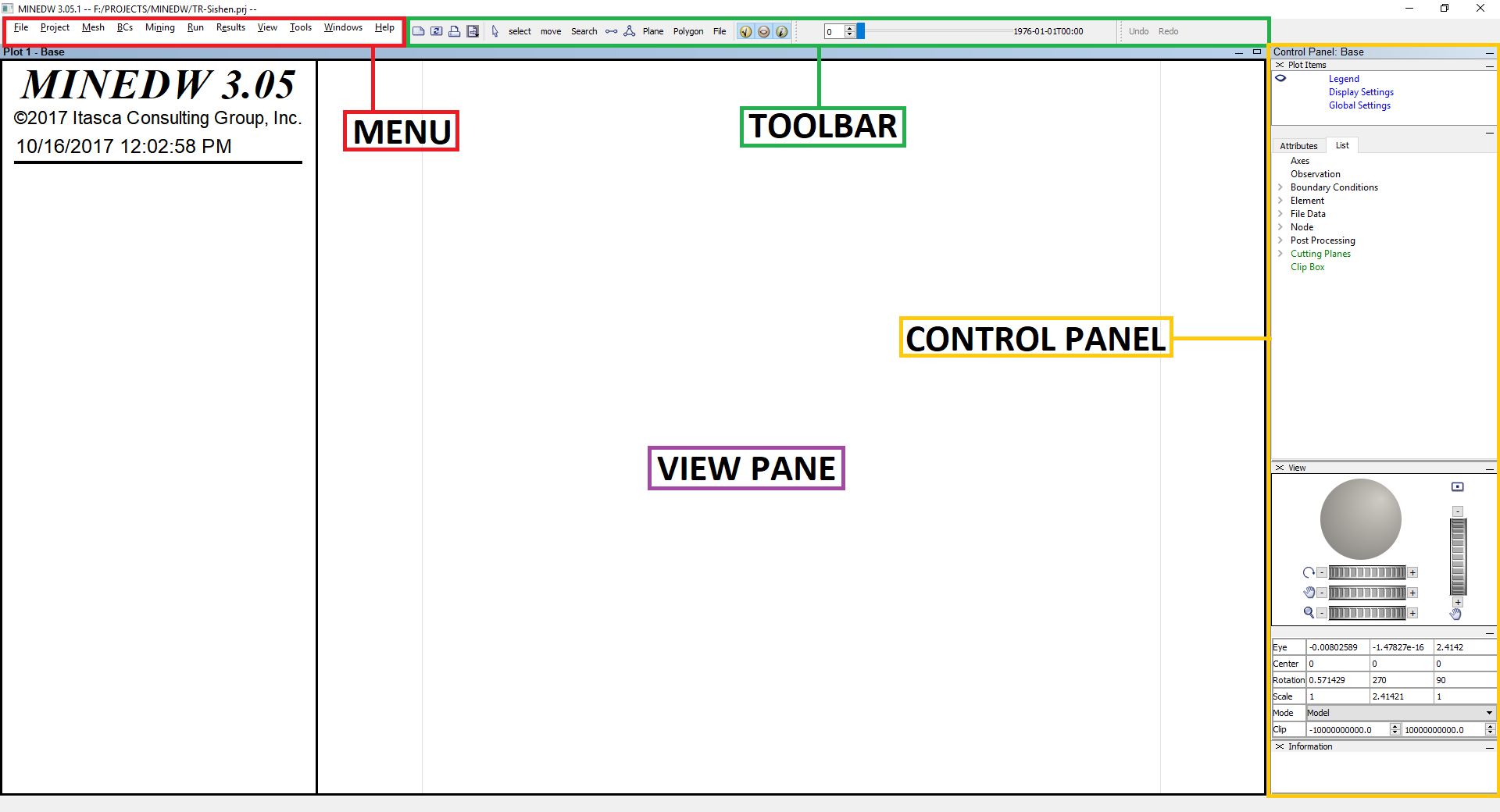
Figure 3.1 The MINEDW main interface
The main interface shown in Figure 3.1 consists of the following components:
View Pane (shown in the purple frame),
Main Menu banner (shown in the red frame),
Toolbar (shown in the green frame), and
Control Panel (shown in the yellow frame).
3.1 View Pane
View Panes are used to store plots and function as a window that can be opened and closed. The View Pane without any plot items is defined as the base View Pane, as shown in Figure 3.1. The base View Pane is a unique View Pane (there is only one) in that it is permanent and cannot be closed, although it can be hidden from view.
The assembly of plot items within a View Pane is performed using the Control Panel, which provides tools that can be used to define the contents of the plot (plot items) and the appearance of those items. A description of the Control Panel is provided in later sections. Plots typically consist of a model mesh, geologic setting, wells, boundary conditions, model outputs, and legend, as shown in Figure 3.2. Note that the Control Panel is turned off in Figure 3.2 in order to illustrate the View Pane.
The plot items in a specific View Pane can be saved in views using the “View” menu. There is no limit to the number of View Panes that can be created and saved. Each saved View Pane is listed under the “View” menu and can be retrieved for viewing or permanently deleted using this menu.
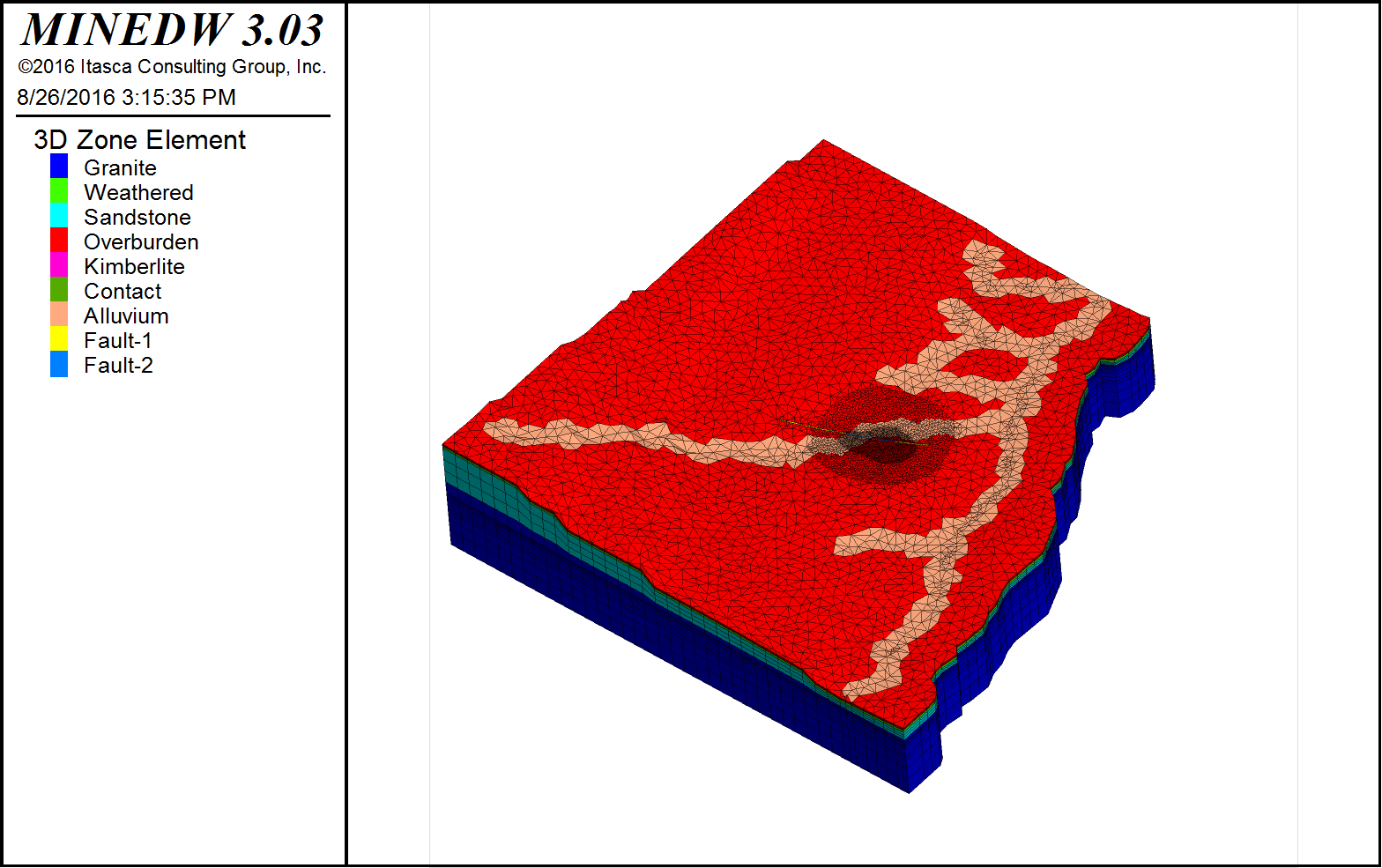
Figure 3.2 Typical layout of a View Pane
3.2 Main Menu
The Main Menu banner in MINEDW includes the major functions of the MINEDW GUI. It contains 11 items: 1) “File,” 2) “Project,” 3) “Mesh,” 4) “BCs,” 5) “Mining,” 6) “Run,” 7) “Results,” 8) “View,” 9) “Tools,” 10) “Windows,” and 11) “Help,” as shown in Figure 3.3.

Figure 3.3 Main Menu banner
3.2.1 The File Menu
The “File” drop-down menu contains the items shown in Figure 3.4. Detailed descriptions of each menu item are also provided in Figure 3.4.
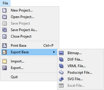
Figure 3.4 “File” drop-down menu
- New Project:
Creates a new project.
- Open Project:
Opens an existing project.
- Save Project:
Saves the current project file. This menu item remains inactive unless there is a change to the modeling components, such as geologic setting, boundary condition, etc.
- Save Project As:
Saves a copy of the current project file using a different file name.
- Close Project:
Closes the project.
- Print Base:
Selects the printing device and prints the base image.
- Export Base:
Exports the base image as a bitmap, .DXF, .VRML, postscript, or .SVG file.
- Import:
Imports a MINEDW project, a FEFLOW data set, or a stereolithography file containing a finite-element mesh. After the “Import” button is clicked, an “Import File” dialog box opens and provides four options. A user can import a MINEDW data-file list (.FEL) that was created for MINEDW model simulations, a MINEDW geometry file (.PST) that was created with the mesh generator from MINEDW 2.10, a geometry file (.STL) that was created using Rhinoceros 3D, a FEFLOW ASCII data file (.FEM), or a FEFLOW ASCII result file (.DAC). If a MINEDW data-set file (.FEL) is used, then all information related to the model—except the results—is imported; however, if a MINEDW geometry file (.PST) is used, then only the geometry and the geologic zone information are imported. Importing model data sets is discussed in detail in Chapter 4.
- Export:
Exports the model in a FEFLOW-supported format that can be imported into FEFLOW for simulation.
- Quit:
Exits MINEDW. When the “Quit” menu item is selected, a warning message appears reminding the user to save the project if it has not been saved, as shown in Figure 3.5. If “Discard” is selected, then all unsaved changes to the model are lost. To save a project or changes to an existing project, the file must be saved before the “Quit” command is used.
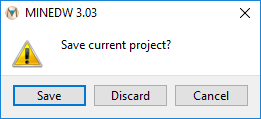
Figure 3.5 The MINEDW “Quit” dialog box
3.2.2 The Project Menu
The “Project” drop-down menu is available from the Main Menu banner and includes the items shown in Figure 3.6.
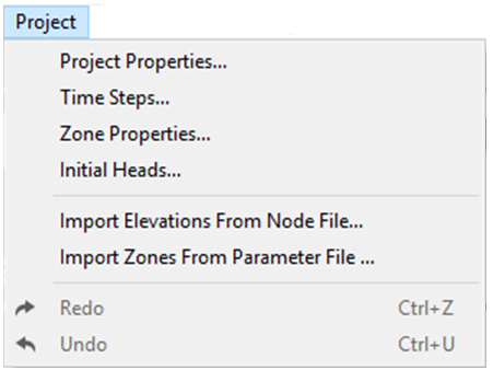
Figure 3.6 The “Project” drop-down menu
- Project Properties:
Contains specifications for the simulation parameters, including units, type of simulation, closure criteria, solver type and solver parameters, and output names. A detailed description of the parameters specified in the “Project Properties” dialog box (Figure 7.1) is provided in Section 7.1.1.
- Time Steps:
Contains information on time steps, the maximum number of time steps, and simulation time steps for model simulations. The parameters specified in the “Setup Time Step” dialog box (Figure 7.2) are described in Section 7.1.2.
- Zone Properties:
Defines the hydraulic properties for each geologic unit simulated in the model. Each zone represents a geologic unit with unique hydraulic properties. A detailed description of material properties is provided in Section 7.3.
- Initial Head:
Defines the initial conditions for hydraulic head in the model. Section 7.5 provides detailed information about the assignment of initial head values.
- Import Elevations from Node File:
Allows for the importing of a node elevation file (node.fem) if changes have been made to node elevations using other editing tools or in another MINEDW model. A brief description on how to import node elevations is provided in Section 7.2.4.
- Import Zones from Parameter File:
Allows for the importing of a zone parameter file (para.fem) if changes have been made to the distribution of hydraulic properties using other editing tools or in another MINEDW model. A detailed description of this function is provided in Section 7.3.1.
- Undo:
Allows the user to undo changes that were made to the groundwater flow model, except in cases where the nodes were changed. A detailed description of this function is provided in Section 3.3.
- Redo:
Allows the user to redo any undone changes to the model, except in cases where the nodes were changed. A detailed description of this function is provided in Section 3.3.
3.2.3 The Mesh Menu
The “Mesh” drop-down menu is available from the Main Menu banner and includes the items shown in Figure 3.7. Detailed information about these menu items is available in Section 7.2.
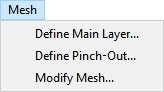
Figure 3.7 The “Mesh” drop-down menu
- Define Main Layer:
This menu is used to create main layers for the model. Main layers are defined as layers that are present throughout the whole model domain. Details about layers can be found in Section 7.2.2.
- Define Pinch-Out:
This menu is used to refine the vertical discretization of the main layers in selected areas. Details about the pinch-out method can be found in Section 7.2.5.
- Modify Mesh:
This menu is used to refine or extend the mesh for a selected area using a boundary line file (.BLN). Details about mesh refinement can be found in Section 7.2.6.
3.2.4 The BCs Menu
The “BCs” menu is a drop-down menu (Figure 3.8) that includes the menu items listed below. Detailed information about these menu items is provided in Section 7.4.
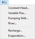
Figure 3.8 The “BCs” menu
- Constant Head:
Menu for assigning constant-head boundary conditions (e.g., boundary head invariable with time, boundary head variable with time, and drain nodes). See Section 7.4.2 for complete details on constant-head assignment.
- Variable Flux:
Menu for assigning variable-flux boundary conditions. See Section 7.4.3 for complete details on the assignment of variable-flux boundaries.
- Pumping Well:
Menu for specifying source-sink terms (e.g., pumping wells). See Section 7.4.4 for complete details on source-sink terms.
- River:
Menu for creating rivers and tributaries. See Section 7.4.5 for complete details on river boundary conditions.
- Recharge:
Menu for assigning recharge zones to the groundwater system. See Section 7.4.6 for complete details on recharge.
- Evaporation:
Menu for assigning the loss of groundwater from a shallow water table due to evapotranspiration and/or evaporation. See Section 7.4.7 for complete details on evaporation.
3.2.5 The Mining Menu
The “Mining” drop-down menu contains the options shown in Figure 3.9. Note that this menu is not active for a steady-state simulation. Details about these menu items can be found in Section 7.6.
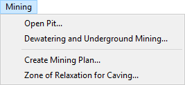
Figure 3.9 The “Mining” drop-down menu
- Open Pit:
This menu is used to simulate open-pit mining in MINEDW. It allows the user to import a previously created mining plan, create new mine plans, set up input parameters for pit-lake simulation, create a ZOR, and define backfilling operations for open pits. Details about this function can be found in Sections 7.6.1 to 7.6.5.
- Dewatering and Underground Mining:
This function is used to construct a simulation involving underground mining. The menu allows the user to create a time-varied hydraulic conductivity file for the model to simulate the changing hydraulic conductivity that results from underground mining operations, freeze-thaw conditions, or other scenarios wherein hydraulic conductivity changes. This menu also allows the user to specify details to simulate the groundwater recovery after the end of mining and to simulate backfilling of the underground excavation if desired. Details about options can be found in Section 7.6.7.
- Create Mining Plan:
Creates a mining file that simulates the progressive excavation of an open-pit mine. Mining plans are then imported into the model using the “Open Pit” menu. Details about creating a mining plan can be found in Section 7.6.1.
- Zone of Relaxation for Caving:
Creates an input file related to caving. Details about ZORs for caving can be found in Section 7.6.6.
3.2.6 The Run Menu
The “Run” drop-down menu contains the items listed in Figure 3.10. Details about these menu items can be found in Section 8.
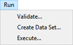
Figure 3.10 The “Run” drop-down menu
- Validate:
Verifies that the groundwater model is correctly defined.
- Create Data Set:
Creates the data files in ASCII format. These files are used in the MINEDW calculation.
- Execute:
Starts the simulation.
3.2.7 The Results Menu
The “Results” drop-down menu contains the items shown in Figure 3.11. Details about these menu items can be found in Section 9.
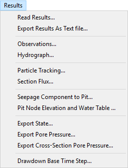
Figure 3.11 The “Results” drop-down menu
- Read Results:
Reads the results from a .PLB file. The .PLB file contains the output of groundwater head at specified time-step intervals from the model simulation. After the results have been read, they can be visualized in the View Pane (described in Section 9.1).
- Export Results As Text File:
This function allows the user to convert a .PLB file (binary file of MINEDW simulation results) to a .PLT file (ASCII file).
- Observations:
Defines the locations and screen intervals of monitoring borehole(s) and the locations of piezometer(s) that can be used to export simulated water levels in ASCII format for external plotting. Details about observations are provided in Section 9.2.
- Hydrograph:
Creates an output data file—in ASCII format and with the file extension .DAT—for plotting a hydrograph based on the observation locations defined in the “Observations” menu. The output data file contains time steps, date and time, and water levels for each observation point. Details about hydrographs are provided in Section 9.3.
- Particle Tracking:
Defines the parameters for particle-tracking simulations and runs the simulations. A detailed explanation of the particle-tracking simulations is provided in Section 9.4.
- Section Flux:
Computes the flux passing through a plane defined by the user using the start and end locations of the plane and vertical height of the plane, as described in detail in Section 9.5.
- Seepage Component to Pit:
Computes seepage to the pit from each geologic unit through time. Details about seepage are provided in Section 9.6.
- Pit Node Elevation and Water Table:
Plots changes in pit node elevation and the water table below the pit node through time for nodes selected by the user. Details about “Pit Node Elevation and Water Table” plots are provided in Section 9.7.
- Export State:
Exports simulation results in either 2-D or 3-D (e.g., x, y, elevation, pressure, drawdown, head, water table, head difference) for the time step selected using the time-step slider. Details about exporting results are discussed in Section 9.8.
- Export Pore Pressure:
Exports pore pressures in 3-D with a specified grid space and dimensions. Details about exporting pore pressures in 3-D are provided in Section 9.9.
- Export Cross-Section Pore Pressure:
Exports pore pressures in 2-D with a specified grid space and section. Details about exporting pore pressures of cross sections are provided in Section 9.10.
- Export Pore Pressure to FLAC3D:
Exports the simulated pore pressure to a FLAC3D format.
- Drawdown Base Time Step:
Defines the time step at which the simulated water level is used as the reference for calculating the drawdown or head difference of a given time. The drawdown is calculated according to the reference time and the selected time step. Detailed information can be found in Section 9.11.
3.2.8 The View Menu
The “View” drop-down menu contains the items shown in Figure 3.12.
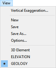
Figure 3.12 The “View” drop-down menu
- Vertical Exaggeration:
Vertically exaggerates the view of plot items. This exaggeration applies to all plot items in the view.
- New:
Creates a new view that can be stored.
- Save:
Saves the current view. View items can be saved with the project file and be reloaded when a project file is loaded in MINEDW. To save the view items that will be reloaded with the project file, the user must also click “Save” in the “File” menu to save the project that contains the saved view items.
- Save As:
Saves a copy of the current view using a different name.
- Options:
Opens “View Options” dialog box, which allows the user to export, import, and delete saved views.
- Listed Views:
If views have been created and saved to the MINEDW .PRJ file, a list of the saved views that are available appears in the drop-down menu (e.g., in Figure 3.12, the listed views are “3D Element,” “Elevation,” and “Geology”). In order to reload these saved view items when reloading a saved project, the project file needs to be saved before termination of the model operation.
3.2.9 The Tools Menu
The “Tools” drop-down menu contains the items listed in Figure 3.13.
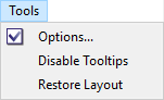
Figure 3.13 The “Tools” drop-down menu
- Options:
The user-specified configuration options in MINEDW are shown in Figure 3.14 and described below. These options are accessed via the “Options” dialog box. The dialog box is divided into areas of functionality that correspond to the buttons shown below.
- Disable Tooltips:
Disables the descriptions that pop up when the mouse hovers on top of a function such as the “Select” tool.
- Restore Layout:
The “Control Panel” Pane, as well as the View Pane, can be moved within the MINEDW window and toggled on or off. To revert back to the default layout of MINEDW, use the “Restore Layout” option.
The “MINEDW Options” dialog box (Figure 3.14) presents the options listed below. The “Display” and “Movie” tabs are discussed in Sections 3.4.1.1 to 3.4.1.3.
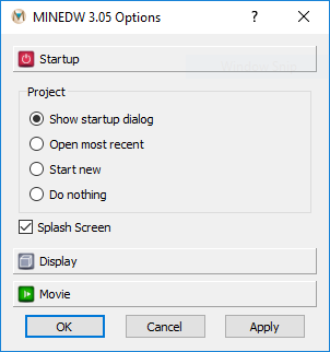
Figure 3.14 The “MINEDW Options” dialog box
- Show Startup Dialog:
After selecting this option (see Figure 3.14) and restarting MINEDW, the “Startup Options” dialog box is displayed (Figure 3.15, below). This enables a user to select what to do next (e.g., “Open Last Project,” “Open Existing Project,” “Create New Project,” or “Cancel”), as shown in Figure 3.15. The “Startup Options” dialog box can be disabled by checking the box at the bottom if the user does not wish to see this option upon startup (see Figure 3.15).
- Open Most Recent:
When selected, this control sets MINEDW to open the most recent project upon startup and to hide the startup dialog box.
- Start New:
When selected, this control sets MINEDW to start a new project upon startup and to hide the startup dialog box.
- Do Nothing:
When selected, this control sets MINEDW to open with no project loaded and to hide the startup dialog box.
- Splash Screen:
When enabled, this control sets the MINEDW splash screen to be shown at the startup of MINEDW.
Figure 3.15 The “Startup Options” dialog box
3.2.10 The Windows Menu
The “Windows” drop-down menu allows the user to toggle the Control Panel and the available plots on or off. By default, it contains the “1 Control Panel” and “2 Plot 1 - Base” file (Figure 3.16). Clicking on the “1 Control Panel” and “2 Plot 1 - Base” options turns the Control Panel and Plot 1 - Base on (as indicated by a check mark) or off. If any plots have been created, they will appear in the “Windows” drop-down menu below “2 Plot 1 - Base” and can be toggled on or off by clicking on the plot name. In Figure 3.16, the plot file named “3 Plot 2 - View004” has been created but is turned off. Clicking on the plot file will turn it on.
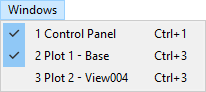
Figure 3.16 The “Windows” drop-down menu
3.3 Toolbar
The MINEDW Main Menu toolbar (Figure 3.18) is found next to the menu banner at the top of the screen. It contains the tools shown in Table 3.1 (below).

Figure 3.18 The MINEDW Main Menu toolbar
Table 3.1 (below) describes the functions of the Main Menu toolbar items.
Table 3.1 The Main Menu Toolbar Item Descriptions
 |
Create New Plot | Creates a new plot in a new View Pane in the active window. |
 |
Regenerate Current Plot (F5) | Refreshes the current plot to reflect the current model data. |
 |
Print the Current Plot (CTRL+P) | Sends the current plot to the printer. |
 |
Export to File | Exports the current plot to a bitmap, .DXF, .VRML, Postscript, or .SVG file format. |
 |
View Mode ‒ Change View Perspective | Changes the cursor to the mode used for basic view manipulation (e.g., rotation, translation, and magnification). |
 |
Select | Changes the cursor to the mode for selecting elements or nodes. |
 |
Move Node | Moves finite-element mesh nodes. |
 |
Search Node/Element | Searches for nodes or elements by node or element number. |
 |
Measure Distance | Calculates the distance between two points. |
 |
Define Plane | Calculates the dip, dip direction, and normal direction of a plane defined by three selected points. |
 |
Create Plane | Creates a cross section using two points defined by the user. |
 |
Select with Polygon | Selects nodes or elements in a desired area defined by a polygon drawn with the mouse pointer. |
 |
Select with Overlay | Selects nodes or elements using a point, polyline, or polygon from “*.DAT,” “*.BLN,” or “*.SHP” files. |
 |
Plot Items | Shows or hides the “Plot Items” control panel. |
 |
View Controls | Shows or hides the “View” control panel. |
 |
View Information | Shows or hides the “Information” control panel. |
To view the desired time step, enter it in the variable field and press [Enter], move the time-step slider (found on the right side, as shown in Figure 3.19), or click the up or down arrow to the desired time step.
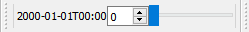
Figure 3.19 Time-step slider
To undo an action, click the “Undo Action” button (Figure 3.20). You can see a list of the actions available to undo in the “Show Undo Stack” window.

Figure 3.20 “Undo,” “Redo,” and “Show Undo Stack” buttons
To redo an action that you undid, click the “Redo Action” button. The action is then reversed.
3.4 Control Panel Pane
The Control Panel displays a plot file created through “Create New Plot.” Each of the plot files is listed under the View Pane. A specific plot file will display in the Control Panel after it is selected.
The attributes of the selected plot are displayed in three sub-panes of the “Control Panel” Pane: 1) “Plot Items,” 2) “View,” and 3) “Information” (as shown in Figure 3.1). The “Plot Item” sub-pane is used to build plots by adding items to the view and specifying their appearance using the available options. The “View” sub-pane provides tools for manipulating the view (e.g., rotation, magnification, and position). The “Information” sub-pane displays information (e.g., location and ID) pertaining to items in the current plot when the cursor is positioned over a specific item in the view. The “Plot Items” and “View” sub-panes are each divided into two sections that can be independently minimized. Each sub-pane set can be displayed or hidden using the control buttons on the toolbar (shown in Figure 3.21).

Figure 3.21 Sub-pane control buttons on the toolbar
3.4.1 Plot Items
Each plot file may consist of several plot items. In MINEDW, plot items are 2-D or 3-D representations of node or element properties and model output such as particle tracks and open-pit seepage. As shown in Figure 3.22 (the MINEDW interface), the “Plot Items” sub-pane contains two sections. The upper section shows the list of plot items, and the lower section offers the option of displaying the attributes (“Attributes”) or selecting other plot items to be displayed (“List”). When a plot item is highlighted, the attributes associated with that item become active. The plot item can be activated (made visible) or deactivated (made invisible) by clicking the ellipse icon to the left of the plot item. Additionally, right-clicking on a plot item brings up a menu that allows the user to activate, deactivate, or delete a plot item from a plot file.
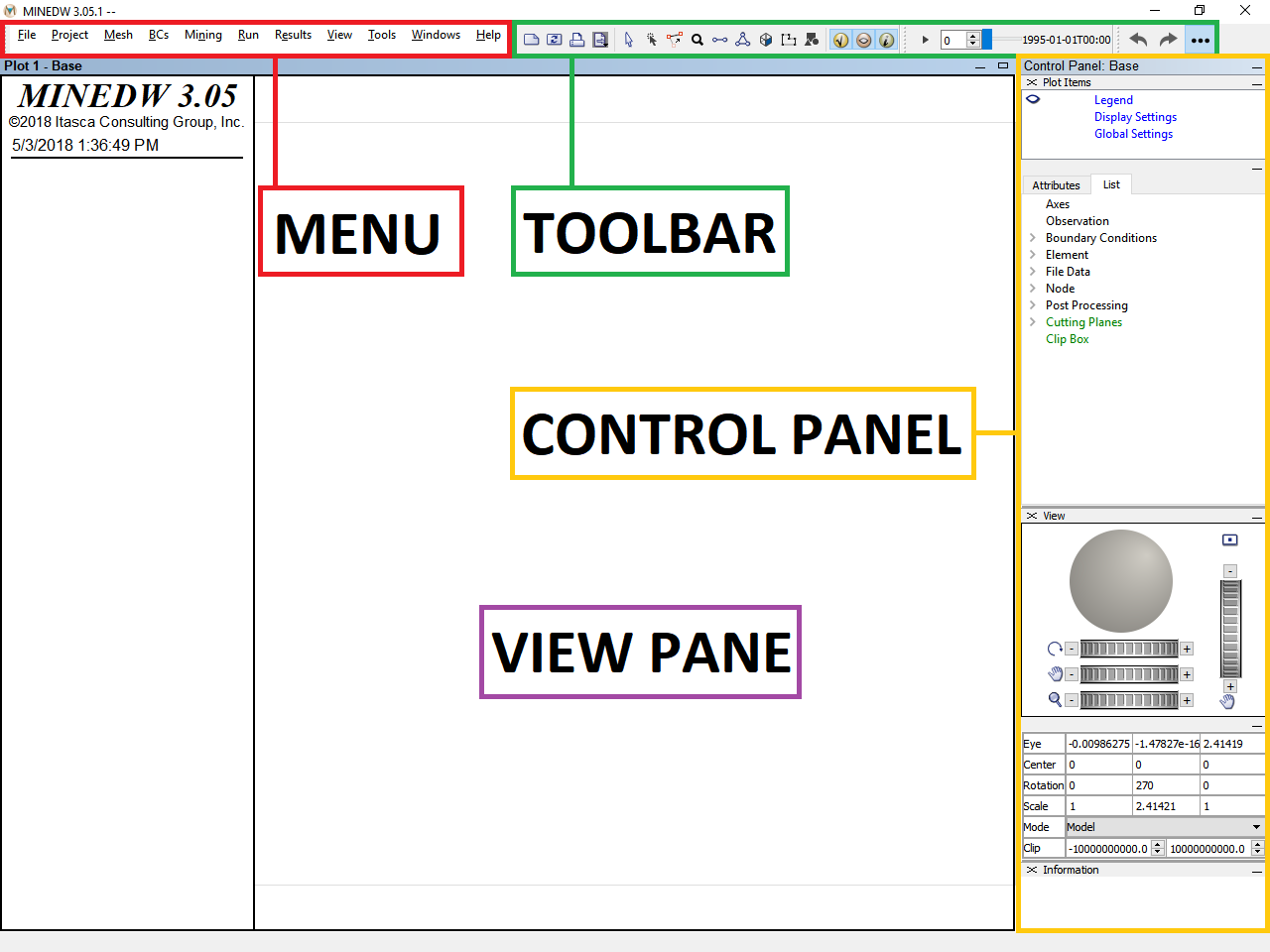
Figure 3.22 The MINEDW main interface
The “Plot Items” sub-pane contains three groups, differentiated by color as shown in Figure 3.23. The first group, which is in blue, contains three special plot items, 1) “Legend,” 2) “Display Settings,” and 3) “Global Settings.” These three plot items are included for all plots. The second group, which is in black, consists of 1) “Axes,” 2) “Observation,” 3) “Boundary Conditions,” 4) “Element,” 5) “File Data,” 6) “Node,” and 7) “Post Processing.” Each item in the second group can be added to a plot. The third group of plot items, which is in green, contains “Cutting Planes” and “Clip Box.” The plot items in the third group can be added to a plot to create different cross-section views through the model domain.
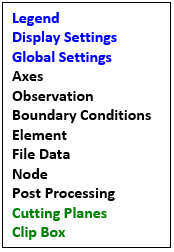
Figure 3.23 MINEDW plot items
3.4.1.1 Legend
“Legend” is a local copy of the legend’s settings that are in effect for the current plot. The legend is displayed on the Legend Pane. On top of the Legend Pane is the MINEDW version and time stamp when the plot was created. There are two alternatives for setting the legend:
Alternative 1 is to set legend attributes before the creation of a plot file. Legend attributes of this alternative are set through the “Options” dialog box under the “Tools” menu on the Main Menu banner. The attributes from Alternative 1 will apply to all new plot files.
Alternative 2 is to set the legend attributes for the currently displayed plot file in the Control Panel Pane. Legend attributes from this alternative only apply to the currently selected plot file and will not affect other plot files or new plot files that will be created.
The attributes associated with legends are described below:
- Placement:
Sets the position of the Legend Panel to one of three preset options: 1) “Left” (side of View Pane), 2) “Right” (side of View Pane), or 3) “Floating” (inside the View Pane).
- Width:
Sets the width of the legend as a percentage of the View Pane containing the plot. The minimum value of width is 25. The width can be increased for all three placement options of the Legend Panel.
- Height:
Sets the height of the Legend Panel as a percentage of the View Pane containing the plot. This setting is only applicable if the “Placement” attribute is set to “Floating.”
- Position:
Specifies the left-side position and bottom position of the plot item as a percentage of the available rendering area. It uses a scale of 0 to 100, in which 0 indicates the bottom-left corner and 100 indicates the top-right corner. Continuous adjustment of the upward vertical position once the top of the Legend Panel reaches the top of the View Pane will reduce the height of the Legend Panel. The “Position” setting is only applicable if the legend “Placement” attribute is set to “Floating.”
- Outline:
Sets the visibility, color, and thickness of the plot item’s outline.
- Heading:
Sets the color of the legend heading.
- Copyright:
Sets the color of the copyright notice in the legend.
- View Info:
Sets the visibility of the current view orientation report in the legend. The report can include the following items—each of which can be selected individually for inclusion in the view info in the legend—“Center,” “Eye,” “Dip/DD/Roll,” “Normal,” “Radius,” and “Projection.” Sub-controls for each of the items are provided for specifying the size, font, style, and color of the text used.
- Step:
This option is inactive in MINEDW.
- Time:
Sets the visibility of the time in the legend. The time used is that at which the view was last modified. The sub-controls provided can specify the size, font, style, and color of the text used to display the time in the legend.
- Customer Title:
This option is not active in MINEDW.
On the “Attributes” tab for the “Legend” item, the legend settings for each of the plot items that the user has added to the current plot are also listed beneath the “Customer Title” attribute. The controls provided can add or remove the plot item from the legend and specify the size, font, style, and color of the text. In the case of plot items that have multiple sub-parts, such as contours or units, the user can add or remove the individual sub-labels from the legend.
3.4.1.2 Display Settings
“Display Settings” is a local copy of the display settings that are in effect for the plot items currently selected. There are two alternatives for setting display:
Alternative 1 is to set display attributes before the creation of a plot file. Display attributes of this alternative are set through the “Options” dialog box under the “Tools” menu on the Main Menu banner. The attributes from Alternative 1 will apply to all new plot files.
Alternative 2 is to set the display attributes for the currently displayed plot file in the Control Panel Pane. Display attributes from this alternative only apply to the currently selected plot file and will not affect other plot files or new plot files that will be created.
The attributes available under “Display Settings” and their descriptions are presented below:
- Name:
Indicates the name of the active view. For all views except the Base View, this control can be used to name or rename the current view.
- Active:
Controls whether the view is active or inactive.
- Auto Update:
Sets the option of whether to auto-update the view while cycling (this is enabled via a checkbox). The interval for updating is found under the “Global Settings” plot item because the interval is the same for all auto-updating views.
- Background:
Sets the background color of the view.
- Outline:
Sets the visibility, color, and thickness of the item’s outline.
- Job Title:
This option is inactive in MINEDW.
- View Title:
Sets the visibility of the title. The sub-controls provided can specify the size, font, style, color, and title displayed in the plot.
- Target:
This option is inactive in MINEDW.
- Movie:
This option is inactive in MINEDW.
3.4.1.3 Global Settings
“Global Settings” is a local copy of the global settings that are in effect for the current plot. The options can be set in the “Plot Items” sub-pane or via the “Options” dialog box found under the “Tools” menu on the Main Menu banner. Changing the settings on the current plot also sets them in the “Options” dialog box and subsequently affects all plot files because these changes are applied globally. The attributes available under “Global Settings” and their descriptions are listed below.
- Vertex Arrays:
Specifies whether vertex arrays are used to draw objects in Open Graphics Library. The default setting is “on.” When using older OpenGL display drivers, disabling this attribute can improve images sometimes. Note that disabling this attribute implies that the vertex buffer objects are also turned off.
- Vertex Buffer Objects:
Determines whether the vertex buffer object OpenGL extension is used (if available). The default setting is “on.” Note that disabling this attribute can improve images when using display drivers that presently report this extension but do not properly support it.
- Interactive1:
This option is inactive in MINEDW.
- Interactive2:
This option is inactive in MINEDW.
- Picking:
This option is inactive in MINEDW.
- Sketch Mode:
Renders the item using a reduced (rather than full) rendering method, which can accelerate response in certain rendering situations (e.g., model rotation).
- Update Interval:
This option is inactive in MINEDW.
- Print Size:
Sets the width and height of the output sent to a printer or to a bitmap file.
- DXF Warning:
Option to display the warning about styling when a .DXF file is exported.
- VRML Warning:
Option to display the warning about styling when a .VRML file is exported.
- Movie:
This option is inactive in MINEDW.
The second group in the “Plot Items” sub-pane consists of “Axes,” “Observation,” “Boundary Conditions,” “Element,” “File Data,” “Node,” and “Post Processing” (shown in MINEDW and Figure 3.23 in black), which can be added to the plot items. These are discussed in more detail in the following sections.
3.4.1.4 Axes
The “Axes” plot item is an interactive orientation indicator that can be displayed as x-, y-, and z-axes or as compass points (easting and northing). The attributes available for axes and their descriptions are given below.
- AutoConf:
Sets the axes display as either x-, y-, and z-axes or as compass points (easting and northing) by clicking the icons shown.
- X-Axis:
The x-axis display with sub-controls for specifying color, draw (in positive, negative, or both directions), “+” label, and “-” label (the axis label in positive and negative directions).
- Y-Axis:
The y-axis display with sub-controls for specifying color, draw (in positive, negative, or both directions), “+” label, and “-” label (the axis label in positive and negative directions).
- Z-Axis:
The z-axis display with sub-controls for specifying color, draw (in positive, negative, or both directions), “+” label, and “-” label (the axis label in positive and negative directions).
- Fixed:
When enabled, this control fixes the axes to a location on the screen. Use the “Screen” attribute to specify the position. When disabled, this control positions the axes in model space.
- Scale:
Specifies a size in percentage units when the axes are fixed.
- Screen:
Specifies the x and y position of the axis center in percentage units (0, 0 = bottom left; 100, 100 = top right) when the axes are fixed.
- Size:
Specifies the axes size in model units when the axes are not fixed.
- Position:
Places the origin of the axis at the x-, y-, and z-position (in model units) specified when the axes are not fixed.
- Font:
Specifies the font, size, and style (e.g., normal, bold, italic) used by the plot item.
- Transparency:
Specifies the plot item’s transparency (70–100). When transparency is toggled off, the point and its label are displayed in opaque state.
- Caption:
When enabled, this control shows the plot item (labeled, described, and enumerated as needed) in the plot legend. The sub-attributes provided are dynamic and contingent on the plot item and its display requirements in the legend. At a minimum, all captions have a “Title” sub-attribute.
3.4.1.5 Observation
The “Observation” plot item includes the display settings for observation wells such as stand pipe with screen (Borehole in Observation) and grouted-in vibrating piezometers (Piezo in Observation). For Piezo, the location of the transducer can also be displayed (Transducer in Observation). The display attributes available for observation wells and their descriptions are given below.
- Map:
This attribute positions, scales, and orients the plot item via the sub-attributes. Sub-attributes include 1) axes, which specify a coordinate substitution to use assuming a standard order of “x, y, z” (“xzy,” for instance, indicates that the y and z coordinates are to be swapped); 2) translate (or offset), which specifies values for x, y, and z plot-item position offsets; and 3) scale, which multiplies the coordinate system by the specified value. These attributes are generally not required to change if the coordinates of the observation points are the same as other plot items of the plot file.
- Colors:
Specifies the number of colors to use on the plot. Includes sub-attributes that enumerate the indexed items to enable specification of color by item. Observation wells are colored by borehole, piezometer, and transducer.
- Line:
Sets the thickness and style of the line(s) used to represent the screen interval of the observation well or piezometer.
- Scale:
Specifies a size in percentage units when the axes are fixed.
- Text:
Displays the labels of the observation wells. By toggling the arrow, the label can be displayed or hidden.
- Transparency:
Specifies the plot item’s transparency (70–100). When transparency is toggled off, the point and its label are displayed in opaque state.
- Caption:
When this control is selected, the plot item is shown (labeled, described, and enumerated as needed) in the plot legend. The sub-attributes provided are dynamic and contingent on the plot item and its display requirements in the legend. At a minimum, all captions have “Title” or “Line” and “Color” sub-attributes. In the case where the Legend Pane is occupied by the legend of other plot items (such as hydrogeologic units), the user can disable the display of selected plot items (such as “Element” or “Node”) to see the caption attributes of the “Observation” plot item.
- Toggle Well:
Provides a list of each observation well that is included in the plot. Individual observation wells can be removed from the View Pane. This function allows the user to include some or all observation wells when exporting a .DXF file from MINEDW.
- Section Distance:
This feature is used in conjunction with a cross-section view. It allows the user to specify which observation locations to display by using a distance. For example, if a user creates a cross section and wishes to display observation locations within 100 meters of the cross-section plane, they would enter “100” in the box next to the attribute label if the coordinate system used in the model is in meters.
3.4.1.6 Boundary Conditions
The “Boundary Conditions” plot item includes the display settings for boundary conditions. The boundary conditions include “Constant Head & Drain,” “Pumping Well,” “River,” and “Variable Flux.” The display attributes available for boundary conditions and their descriptions are given below. Detailed information about the boundary conditions can be found in Section 7.4.
Constant Head & Drain
- Map:
This attribute positions, scales, and orients the plot item via the sub-attributes. Sub-attributes include 1) axes, which specify a coordinate substitution to use assuming a standard order of “x, y, z” (“xzy,” for instance, indicates that the y and z coordinates are to be swapped); 2) translate (or offset), which specifies values for x, y, and z plot-item position offsets; and 3) scale, which multiplies the coordinate system by the specified value. These attributes are generally not required to change if the coordinates of the constant head or drain are the same as other plot items of the plot file.
- Scale:
Specifies the size of the plot item.
- Groups:
Constant-head boundary nodes can be grouped to represent a specified hydrogeologic component, such as a surface-water body, an underground drift, or a pumping well. Each group of constant-head nodes can be presented in a different color in MINEDW.
- Text:
This attribute sets the font style, text size, and text style of the labels of the boundary conditions displayed in the View Pane.
- Transparency:
Specifies the plot item’s transparency (70–100). The minimum value for transparency setting is 70. When the transparency is toggled off, the plot item is displayed in opaque state.
- Caption:
When enabled, the plot item is shown (labeled, described, and enumerated as needed) in the plot legend. The sub-attributes provided are dynamic and contingent on the plot item and its display requirements in the legend. At a minimum, all captions have “Title” or “Line” and “Color” sub-attributes. In the case where the Legend Pane is occupied by the legend of other plot items (such as hydrogeologic units), the user can disable the display of selected plot items (such as “Element” or “Node”) to see the caption attributes of the “Boundary Conditions” plot item.
- Maximum Flux:
By specifying a value, the user can specify the upper limit of flux values to display. Flux values larger than the specified value will not be displayed.
- Excluded Flux:
By specifying a value, the user can exclude certain flux values from display.
- Dynamic:
This option only applies to “Constant Head & Drain” boundary conditions and is used to visualize boundary conditions that become active/inactive at different times through the model simulation.
Pumping Well
There are three types of pumping wells in MINEDW:
Rate: The well is simulated with the assigned pumping rate.
Head: The well is simulated as a specified head and the pumping rate is derived from the model simulation.
LPE: The well is simulated with the assigned lowest pumping elevation (LPE). If the simulated water level of the well reaches the LPE, the active pumping will be switched to passive draining to prevent the drying up of the well and pump.
- Map:
Same as in “Constant Head & Drain.”
- Color:
Each type of pumping well is presented in a different color. Deselecting a specific type will remove that type of well from the View Pane and Legend Pane.
- Line:
Sets the thickness and style of the lines used to represent the well depth.
- Scale:
When the “Scale” box is checked, increasing the scale value will increase the size of the dot of each well. Unchecking the “Scale” box will display the default size of the dot.
- Text:
Same as in “Constant Head & Drain.”
- Transparency:
Same as in “Constant Head & Drain.”
- Caption:
Same as in “Constant Head & Drain.”
- Toggle Well:
This feature is used to toggle the display of each well.
- Section Distance:
This feature is used in conjunction with a cross-section view and only applies to the “Pumping Well” plot item. It allows the user to specify which pumping well to display by using a distance in model units. For example, if a user creates a cross section and wishes to display pumping wells within 100 meters of the cross-section plane, they would enter “100” in the box next to the attribute label.
Variable Flux
- Map:
Same as in “Constant Head & Drain.”
- Scale:
Same as in “Constant Head & Drain.”
- Transparency:
Same as in “Constant Head & Drain.”
- Caption:
Same as in “Constant Head & Drain.”
- Flux View:
Same as in “Constant Head & Drain.”
- File:
Same as in “Constant Head & Drain.”
- Minimum Flux:
Same as in “Constant Head & Drain.”
- Maximum Flux:
Same as in “Constant Head & Drain.”
- Excluded Flux:
Same as in “Constant Head & Drain.”
3.4.1.7 Element
The “Element” plot items include 2-D and 3-D plot items that can be used to display hydrogeologic properties of elements. These properties include geologic zones, recharge, evaporation, hydraulic properties, and time-varied conductivity. “Element” plot items also include the “Pinch-Out” plot item, which can be used to view and assign pinch-outs in the model.
- 2D Plane:
Displays element information for the geologic zone (“Zone”), recharge (“Recharge”), or evaporation (“Evaporation”) in 2-D plane view.
- 3D Element:
Displays element information for the hydrogeologic zone in 3-D.
- Pinch-Out:
Allows the user to create areas of refined vertical discretization and display these areas.
- Properties:
Displays hydraulic properties (K:sub:`x`, K:sub:`y`, K:sub:`z`, S:sub:`y`, and S:sub:`s`) in 3-D.
- Time-Varied Conductivity:
Displays the ZOR created for an open pit or cave zone for underground mining in the “Mining” menu.
The attributes related to these plot items are described below.
2D Plane
- Color By:
Specifies which attribute is used for the plot. The attributes include “Zone,” “Recharge,” and “Evaporation.”
- Layer:
Indicates which layer of the model to display on the plot.
- Map:
This attribute positions, scales, and orients the plot item via the sub-attributes. Sub-attributes include 1) axes, which specify a coordinate substitution to use assuming a standard order of “x, y, z” (“xzy,” for instance, indicates that the y and z coordinates are to be swapped); 2) offset (or translate), which specifies values for x, y, and z plot-item position offsets; and 3) scale, which multiplies the coordinate system by the specified value.
- Colors:
Allows the user to specify the colors to be used in the plot. This attribute also allows the user to select which items they wish to display in the plot by activating the checkbox next to the item.
- Fill:
Specifies whether polygons rendered by a plot item should be filled.
- Wireframe:
Specifies whether the plot item should be displayed with a wireframe and determines the color and the line thickness of the displayed wireframe.
- Wire Trans:
Not active.
- Cull Backface:
Specifies whether backface culling is enabled. When set to “On,” the backfaces of polygons are not rendered (it is often necessary to disable this function to see the far side of some cut-plane plots).
- Lighting:
Option to turn lighting on or off. Lighting provides depth to the plot item because it creates natural shadows.
- Offset:
Specifies settings for the OpenGL polygon offset. If the polygons are rendered poorly, then setting these values close to zero might improve performance. The first value specifies a scale factor to create a variable-depth offset for each polygon; the second value creates a constant-depth offset.
- Cutline:
Specifies the line thickness of lines plotted on a cutting plane, with a range of 1 to 10.
- Cutplane:
This option is only active when a cutplane plot item is added to the plot view. The options for “Cutplane” are “On,” “Front,” and “Back,” which turn on the cutplane, make the model domain on the front of the cutplane visible, and make the model domain on the back of the cutplane visible, respectively. In order to show the entire plane, the “Cull Backface” option should be unchecked.
- Clip Box:
Specifies which of the clip box items available in the current view to apply to the current plot item. This option is only active when a clip box plot item is added to the plot view.
- Transparency:
Specifies the plot item’s transparency (70–100). When unchecked, the plot item is displayed in opaque state.
- Caption:
When enabled, the plot item is shown (labeled, described, and enumerated as needed) in the plot legend. The sub-attributes provided are dynamic and contingent on the plot item and its display requirements in the legend. At a minimum, all captions have “Title” or “Colors” and “Label” sub-attributes.
3D Plane
- Layer:
Same as in “2D Plane.”
- Map:
Same as in “2D Plane.”
- Zones:
Allows the user to specify which of the geologic zones are visible in the plot.
- Fill:
Same as in “2D Plane.”
- Wireframe:
Same as in “2D Plane.”
- Wire Trans:
Same as in “2D Plane.”
- Cull Backface:
Same as in “2D Plane.”
- Lighting:
Same as in “2D Plane.”
- Offset:
Same as in “2D Plane.”
- Cutline:
Same as in “2D Plane.”
- Cutplane:
Same as in “2D Plane.”
- Clip Box:
Same as in “2D Plane.”
- Transparency:
Same as in “2D Plane.”
- Caption:
Same as in “2D Plane.”
Pinch-Out
- Map:
Same as in “2D Plane.”
- Colors:
Change the color of each pinch-out zone.
- Fill:
Same as in “2D Plane.”
- Wireframe:
Same as in “2D Plane.”
- Wire Trans:
Same as in “2D Plane.”
- Cull Backface:
Same as in “2D Plane.”
- Lighting:
Same as in “2D Plane.”
- Offset:
Same as in “2D Plane.”
- Cutline:
Same as in “2D Plane.”
- Cutplane:
Not active.
- Clip Box:
Not active.
- Transparency:
Same as in “2D Plane.”
- Caption:
Same as in “2D Plane.”
Properties
- Color By:
Select a hydraulic parameter for display.
- Layer:
Same as in “2D Plane.”
- Map:
Same as in “2D Plane.”
- Contour:
Provides sub-attributes for controlling contour display. These are 1) “Ramp,” which defines the color ramp to use (grayscale, rainbow, etc.); 2) “Maximum,” which specifies (or automatically calculates) the maximum value (right-hand end of the ramp); 3) “Minimum,” which specifies (or automatically calculates) the minimum value (left-hand end of the ramp); 4) “Interval,” which specifies (or automatically calculates) the interval between colors on the ramp; 5) “Reversed,” which inverts the display of the maximum and minimum values relative to the ramp; 6) “Below,” which specifies (or automatically selects) the color to use for displaying values that are less than those specified by “Minimum”; and 7) “Above,” which specifies (or automatically selects) the color to use for displaying values that are greater than those specified by “Maximum.” This attribute is only available for the “Properties” plot item.
- Fill:
Same as in “2D Plane.”
- Wireframe:
Same as in “2D Plane.”
- Wire Trans.:
Same as in “2D Plane.”
- Cull Backface:
Same as in “2D Plane.”
- Lighting:
Same as in “2D Plane.”
- Offset:
Same as in “2D Plane.”
- Cutline:
Same as in “2D Plane.”
- Cutplane:
Same as in “2D Plane.”
- Clip Box:
Same as in “2D Plane.”
- Transparency:
Same as in “2D Plane.”
- Caption:
Same as in “2D Plane.”
Time-Varied Conductivity
- Map:
Same as in “2D Plane.”
- Colors:
Change the color of each pinch-out zone.
- Fill:
Same as in “2D Plane.”
- Wireframe:
Same as in “2D Plane.”
- Wire Trans.:
Same as in “2D Plane.”
- Cull Backface:
Same as in “2D Plane.”
- Lighting:
Same as in “2D Plane.”
- Offset:
Same as in “2D Plane.”
- Cutline:
Same as in “2D Plane.”
- Cutplane:
Same as in “2D Plane.”
- Clip Box:
Same as in “2D Plane.”
- Transparency:
Same as in “2D Plane.”
- Caption:
Same as in “2D Plane.”
3.4.1.8 File Data
The “File Data” item contains options for importing source files that were not generated by the MINEDW program. These options are described below.
BLN (Boundary Line File)
The “BLN” (boundary line) plot item is used to import and display a .BLN file. The attributes available for “BLN” and their descriptions are provided below.
- File:
Clicking on the plus sign (+) opens the “Select BLN file” dialog box. Once loaded, the file name is shown in this attribute.
- Project to Surface:
Projects the BLN lines to the ground surface.
- Map:
This attribute positions, scales, and orients a plot item via the sub-attributes. Sub-attributes include 1) axes, which specify a coordinate substitution to use assuming a standard order of “x, y, z” (“xzy,” for instance, indicates that the y and z coordinates are to be swapped); 2) offset (or translate), which specifies values for x, y, and z plot-item position offsets; and 3) scale, which multiplies the coordinate system by the specified value.
- Colors:
Specifies the color of the BLN lines.
- Line:
Specifies the thickness of the BLN lines.
- Text:
Specifies the font used for labels.
- Transparency:
Specifies the plot item’s transparency (0 = solid, 100 = invisible).
- Caption:
When enabled, the plot item is shown (labeled, described, and enumerated as needed) in the plot legend. The sub-attributes provided are dynamic and contingent on the plot item and its display requirements in the legend. At a minimum, all captions have “Title” or “Colors” and “Label” sub-attributes.
DXF (Drawing Exchange Format)
This plot item is used to import and display a .DXF file in the View Pane. The attributes available for this option and their descriptions are provided below.
- File:
The plus sign (+) available for this attribute can be used to display a “Select DXF data file” dialog box for selecting the .DXF file to load. Once loaded, the file name is shown in this attribute.
- Layers:
Indicates the number of layers in a .DXF plot item and provides sub-attributes to control the visibility and color for each layer in the .DXF.
- Map:
This control positions, scales, and orients the plot item via the sub-attributes. Sub-attributes include 1) axes, which specify a coordinate substitution to use assuming a standard order of “x, y, z” (“xzy,” for instance, indicates that the y and z coordinates are to be swapped); 2) offset (or translate), which specifies values for x, y, and z plot-item position offsets; and 3) scale, which multiplies the coordinate system by the specified value.
- Faces:
Provides controls for rendering the faces of the plot item, including fill, wireframe, wireframe transparency, cull backface, lighting, offset, and cutline.
- Cut Faces:
Specifies the thickness and style used to render the outline of faces on the plot item. A plane should be generated before the operation of this attribute.
- Cutplane:
Specifies which of the cutplanes available in the current view to apply to the current plot item. A plane should be generated before the operation of this attribute.
- Clip Box:
Specifies which of the clip box items available in the current view to apply to the current plot item.
- Transparency:
Specifies the plot item’s transparency (0 = solid, 100 = invisible).
- Caption:
When enabled, the plot item is shown (labeled, described, and enumerated as needed) in the plot legend. The sub-attributes provided are dynamic and contingent on the plot item and its display requirements in the legend. At a minimum, all captions have “Title” or “Colors” and “Label” sub-attributes.
- To Zone:
Selects elements contained within a 3-D .DXF object based on the criteria selected by the user and assigns them to the selected group (options are “To Zone,” “Select With,” “Element Selected When Including,” and “Layer Thickness”).
- To Data File:
Saves the .DXF file to a text file format that can be used for creating an open-pit mine plan.
ESRI Shapefile (SHP)
This plot item is used to import a shapefile (.SHP), a common ArcGIS© file format, to the current view. A shapefile is a popular geospatial vector data format for geographic information systems software. Shapefiles spatially describe geometries—points, polylines, and polygons. A shapefile is actually a group of several files, three of which are required to form a valid set. A valid shapefile set contains at least a main file (.SHP), a dBASE file (.DBF), and an index file (.SHX). The main file contains spatial information about features (e.g., coordinates along a line or polygon), the dBASE file contains a table of attributes related to those spatial features (e.g., the name of a feature or some measurement taken at a feature), and the index file indexes the byte-location of features within a .SHP file. The attributes available for this option and their descriptions are provided below.
- File:
Use the plus sign (+) available for this attribute to display the “Select SHP file” dialog box to select which .SHP files to load. Once loaded, the file name is shown in this attribute.
- Attribute Table:
Displays the contents of the dBASE file. A dBASE file contains a table of attributes associated with the features defined in a shapefile.
- Coordinate Info:
Displays the contents of a .PRJ file (a .PRJ shapefile is not related to the .PRJ file created by MINEDW). A .PRJ file contains information about the coordinate system and projection in which the shapefile features are defined. A .PRJ file may or may not be present.
- Group by:
Specifies an attribute of the dBASE file with which to group features. Each group is given a unique color and label in the legend and view. To display all features as separate entities, select the last item (Record ID) from the drop-down menu.
- Label by:
Specifies an attribute of the dBASE file by which to label features within the view. Because an apparently single feature may be defined in a shapefile as several features (e.g., a line composed of line segments), duplicate labels may appear.
- Project to Surface:
Projects the .SHP file to the ground surface.
- Symbol:
Specifies the symbol to represent the data.
- Scale:
Specifies the size of the symbol.
- Colors:
Specifies the colors of features in the shapefile.
- Line:
Specifies line thickness of the data.
- Map:
This control positions, scales, and orients the plot item via the sub-attributes. Sub-attributes include 1) axes, which specify a coordinate substitution to use assuming a standard order of “x, y, z” (“xzy,” for instance, indicates that the y and z coordinates are to be swapped); 2) offset (or translate), which specifies values for x, y, and z plot-item position offsets; and 3) scale, which multiplies the coordinate system by the specified value.
- Text:
Specifies the font used for labels.
- Transparency:
Specifies the plot item’s transparency (70–100). The lowest value for transparency is 70. When unchecked, the plot item is displayed in opaque state.
- Caption:
When enabled, the plot item is shown (labeled, described, and enumerated as needed) in the plot legend. The sub-attributes provided are dynamic and contingent on the plot item and its display requirements in the legend. At a minimum, all captions have “Title” or “Colors” and “Label” sub-attributes.
Point Data
This plot item is used to display x, y, and z data as points. The attributes available for this option and their descriptions are given below.
- File:
Use the plus sign (+) available for this attribute to display the “Select Data File” dialog box to select which .DAT files to load. Once loaded, the file name is shown in this attribute.
- Project to Surface:
Projects the .DAT file to the ground surface.
- Text:
Specifies the font used for labels.
- Map:
This control positions, scales, and orients the plot item via the sub-attributes. Sub-attributes include 1) axes, which specify a coordinate substitution to use assuming a standard order of “x, y, z” (“xzy,” for instance, indicates that the y and z coordinates are to be swapped); 2) offset (or translate), which specifies values for x, y, and z plot-item position offsets; and 3) scale, which multiplies the coordinate system by the specified value.
- Scale:
Specifies the size of the symbol.
- Colors:
Specifies the color of the points.
- Transparency:
Specifies the plot item’s transparency (0 = solid, 100 = invisible).
- Caption:
When enabled, the plot item is shown (labeled, described, and enumerated as needed) in the plot legend. The sub-attributes provided are dynamic and contingent on the plot item and its display requirements in the legend. At a minimum, all captions have “Title” or “Colors” and “Label” sub-attributes.
3.4.1.9 Node
The “Node” plot item includes 2-D and 3-D plots that are related to properties of finite-element nodes. These properties include nodal elevation, groundwater head, pore pressure, drawdown at a given time, and head difference for two different dates in both 2-D and 3-D.
- 2D Contour:
Displays groundwater head, pressure, elevation, head difference, water table, and drawdown in 2-D.
- 3D Contour:
Displays groundwater head, pressure, elevation, and head difference in 3-D.
- Isoline:
Displays isolines for elevation, pore pressure, head, head difference, water table, and drawdown.
- Isosurface:
Displays isosurfaces for elevation, head, pore pressure, and head difference.
The attributes related to these four plot items are described below.
2D Contour and 3D Contour
- Color By:
Specifies which attribute is used for the plot.
- Layer:
Specifies which layer of the model is displayed on the plot.
- Map:
This attribute positions, scales, and orients the plot item via the sub-attributes. Sub-attributes include 1) axes, which specify a coordinate substitution to use assuming a standard order of “x, y, z” (“xzy,” for instance, indicates that the y and z coordinates are to be swapped); 2) offset (or translate), which specifies values for x, y, and z plot-item position offsets; and 3) scale, which multiplies the coordinate system by the specified value.
- Contour:
Provides sub-attributes for controlling contour display. These are 1) “Ramp,” which defines the color ramp to use (grayscale, rainbow, etc.); 2) “Maximum,” which specifies (or automatically calculates) the maximum value (right-hand end of the ramp); 3) “Minimum,” which specifies (or automatically calculates) the minimum value (left-hand end of the ramp); 4) “Interval,” which specifies (or automatically calculates) the interval between colors on the ramp; 5) “Reversed,” which inverts the display of the maximum and minimum values relative to the ramp; 6) “Below,” which specifies (or automatically selects) the color to use for displaying values that are less than those specified by “Minimum”; and 7) “Above,” which specifies (or automatically selects) the color to use for displaying values that are greater than those specified by “Maximum.”
- Fill:
Specifies whether polygons rendered by a plot item should be filled.
- Line:
Sets the thickness and color of the lines used to represent the plot item. The attribute is only available for the Isoline plot item.
- Wireframe:
Specifies whether the plot item should display with a finite-element mesh wireframe as well as the color and the line thickness of the wireframe.
- Wire Trans:
Specifies the wireframe’s transparency (0 = solid, 100 = invisible).
- Cull Backface:
Specifies whether backface culling is enabled. When this setting is enabled, the backfaces of polygons are not rendered (it often is necessary to turn off this feature to see the far side of some cutplane plots).
- Lighting:
Enables the lighting.
- Offset:
Specifies settings for the OpenGL polygon offset. If the polygons are rendered poorly, then setting these values close to zero might improve performance. The first value is a factor that specifies a scale factor to create a variable-depth offset for each polygon; the second value is used to create a constant-depth offset.
- Cutline:
Specifies the line thickness of lines plotted on a cutting plane.
- Cutplane:
Option for displaying the model domain in front of or behind (or both) a cross-section plane. This option is useful when orienting the cross-section plane.
- Clip Box:
Specifies which of the clip box items available in the current view to apply to the current plot item.
- Transparency:
Specifies the plot item’s transparency (70–100). The lowest value for transparency is 70. When unchecked, the plot item is displayed in opaque state.
- Caption:
When enabled, the plot item is shown (labeled, described, and enumerated as needed) in the plot legend. The sub-attributes provided are dynamic and contingent on the plot item and its display requirements in the legend. At a minimum, all captions have “Title” or “Colors” and “Label” sub-attributes.
Isoline
The attributes of “Isoline” are the same as those described in the “2D Contour and 3D Contour” section with the exception of the following:
- Cutplane:
Though a cutplane is not very meaningful for “Isoline,” a user can generate a plane through the “Cutplane” option from “List.”
- Clip Box:
This operation is functional but does not provide meaningful display.
Isosurface
The attributes of “Isosurface” are the same as those described in the “2D Contour and 3D Contour” section with the exception of “Cutplane.” A cutplane can only be created through the “Plane” option under “Cutting Planes” in “List.”
3.4.1.10 Post Processing
- Particle Tracking:
Displays particle-tracking results (Section 9.4).
- Pit Flux:
This option can be used to display the seepage that occurs at the pit wall, which is recorded by MINEDW during the model simulation in the file with a .SEP extension (Section 9.6).
Particle Tracking
To operate the attributes related to particle tracking, a particle-tracking result should be inputted as a MINEDW plot item. The attributes related to the “Particle Tracking” plot item are described below.
- File:
The icon next to the “File” attribute opens a dialog box that is used to import particle tracks.
- Arrow Scale:
This attribute controls the size of the arrow displayed on the particle tracks that indicate direction. It does not apply to the last time step.
- ColorByMag:
The magnitude of the velocity along the displayed particle tracks can be shown by using this attribute. This attribute allows the selection of a number of color ramps and allows the “Maximum,” “Minimum,” and “Interval” to be defined. It does not apply to the last time step.
- Map:
This attribute positions, scales, and orients the plot item via the sub-attributes. Sub-attributes include 1) axes, which specify a coordinate substitution to use assuming a standard order of “x, y, z” (“xzy,” for instance, indicates that the y and z coordinates are to be swapped); 2) offset (or translate), which specifies values for x, y, and z plot-item position offsets; and 3) scale, which multiplies the coordinate system by the specified value.
- Colors:
This attribute can be used to control the display color of particle tracks.
- Line:
Sets the thickness and style of the lines used to represent the “Particle Tracking” plot item.
- Transparency:
Specifies the plot item’s transparency (0 = solid, 100 = invisible).
- Caption:
When enabled, the plot item is shown (labeled, described, and enumerated as needed) in the plot legend. The sub-attributes provided are dynamic and contingent on the plot item and its display requirements in the legend. At a minimum, all captions have “Title” or “Colors” and “Label” sub-attributes.
- Scale:
Controls the size of the displayed seepage point.
- Colors:
This attribute can be used to control the display color of seepage points.
- Transparency:
The same as in “Particle Tracking.”
- Caption:
The same as in “Particle Tracking.”
- Flux View:
This option enables the display of flux values from the “Pit Flux” boundary conditions using both color and marker size to represent the relative magnitudes of flux.
- File:
The icon next to the “File” attribute opens a dialog box that is used to import a pit-flux file.
- Minimum Flux:
Sets the minimum absolute flux value to display using the “Pit Flux” boundary condition.
- Maximum Flux:
Sets the maximum absolute flux value to display using the “Pit Flux” boundary condition.
- Excluded Flux:
Option to enable the display of flux values outside of the specified minimum and maximum flux values.
3.4.1.11 Cutting Planes
The third “Plot Items” group consists of “Cutting Planes” and “Clip Box.” “Cutting Planes,” contains “Plane,” “Wedge,” and “Octant.” Both “Cutting Planes” and “Clip Box” are displayed in green in MINEDW. These items are similar to plot items (and are handled as plot items) in that they are independent objects appearing in the plot. They are distinct from plot items in that they are applied to one or more plot items for the purpose of visualization and, as such, are dependent on plot items. For example, a cutplane can be defined as part of a plot, but until it is applied to at least one plot item, its rendering is incomplete and is not visible in the View Pane.
The “Cutting Planes” group contains three items: 1) “Plane,” 2) “Wedge,” and 3) “Octant.” The function of each item is described below:
- Plane:
The plane can be applied to plot items to “slice” them into 2-D. A plane is manipulated using its “Origin,” which can be repositioned to move the cutplane, and the visible surface of the plane itself can be rotated in the View Pane to view different aspects of the plane.
- Wedge:
The wedge cutplane can be applied to plot items to “slice” the model into a wedge shape that is defined by two planes joined along an origin. The plane is manipulated using its “Origin,” which can be changed to reposition the location of the cutplane.
- Octant:
The octant cutplane provides a cubical cutplane that can be applied to plot items to “slice” them in three orthogonal directions simultaneously. The plane is manipulated using its “Origin,” which can be repositioned. The visible surface of the plane itself can be dragged to rotate the plane three-dimensionally.
The attributes available for cutting planes and their descriptions are given below.
Plane
- Name:
Sets or indicates the name of the cutplane. This name is used to label the cutplane as it is listed in the “Plot Items” list, on the “Cutplane” selector in the attribute list for all plot items (under the “Cutplane” attribute), and in the legend (if its “Caption” attribute is enabled).
- Origin:
The origin of the plane.
- Normal (1, 2, 3):
Defines the orientation of the indicated cutplane via a normal vector.
- Dip/DD (1, 2, 3):
Sets the dip and dip direction, respectively, of the selected plane. There are two of these controls on a wedge and three on an octant; they are labeled with numerals (e.g., 1, 2, 3).
- Snap View:
Snaps the view to a perpendicular orientation so that the user sees the side of the plane. One click will display normal orientation; the second click will display the view in reverse orientation.
- Move Normal:
Moves the cutting plane along the normal direction. The user can enter the interval of each move or use the default value.
- Target:
This attribute is not used in “Move Normal.”
- Caption:
When enabled, the plot item is shown (labeled, described, and enumerated as needed) in the plot legend. The sub-attributes provided are dynamic and contingent on the plot item and its display requirements in the legend. At a minimum, all captions have “Title” or “Line” and “Color” sub-attributes.
Wedge
- Name:
Same as in “Plane.”
- Origin:
The origin of the wedge plane.
- Normal 1:
Defines the orientation of one side of the wedge plane via a normal vector.
- Dip 1/DD 1:
Sets the dip and dip direction of one side of the wedge plane.
- Snap View:
Same as in “Plane” for one plane of the wedge.
- Normal 2:
Defines the orientation of the other side of the wedge plane via a normal vector.
- Dip 2/DD 2:
Sets the dip and dip direction of the other side of the wedge plane.
- Snap View:
Same as in “Plane” for the other plane of the wedge.
- Wedge Angle:
Sets the angle of the wedge cutting plane.
- Caption:
Same as in “Plane.”
Octant
The attributes of “Octant” are the same as in “Wedge” with the following exceptions:
There are three attributes of “Normal,” “Dip/DD,” and “Snap View.”
There is no “Wedge Angle.”
3.4.1.12 Clip Box
When applied to a plot item, the “Clip Box” control constrains the display of the plot item according to its size, position, and orientation. It is similar to a cutplane in that it is applied to plot items and, although a view can have multiple clip boxes in it, only one clip box can be applied to a given plot item at a time. Both a cutplane and clip box can be applied to a plot item simultaneously. The attributes available for the “Clip Box” controls and their descriptions are given below.
- Name:
Sets or indicates the name of the clip box. This name is used to label the clip box as it is listed in the “Plot Items” list, on the “Clip Box” selector in the attribute list for all plot items (under the “Clip Box” attribute), and in the legend if its “Caption” attribute is enabled.
- Center:
Sets the position of the plot item’s center in model units.
- Dip:
Sets the dip of the clip box.
- Dip Dir:
Sets the dip direction of the clip box.
- Clip Axis (1, 2, 3):
Activates a specified axis that will determine the direction of clipping. If “Clip Axis 1” is selected, clipping only occurs along the x direction.
- Axis Radii:
Specifies the radius of clip axis 1, clip axis 2, and clip axis 3, respectively, away from the current center.
- Axis Offsets:
Specifies the offset from the center of each of the three axes.
- Interactive:
This option is not active in MINEDW.
- Caption:
When enabled, the plot item is shown (labeled, described, and enumerated as needed) in the plot legend. The sub-attributes provided are dynamic and contingent on the plot item and its display requirements in the legend. At a minimum, all captions have a “Title” sub-attribute.
3.4.2 View
The “View” sub-pane of the “Control Panel” Pane (Figure 3.24) is discussed in this section. As shown in Figure 3.24, the “View” sub-pane is divided into two sections that can be minimized independently and provides tools for manipulating (i.e., rotating, magnifying, positioning) the view. The functions available in the “View” sub-pane are shown in Figure 3.24 and are described below.
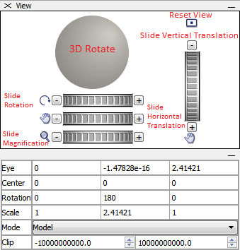
Figure 3.24 A “View” pane and sub-panes
- 3D Rotate:
Use the roller tool to rotate the view in 3-D.
- Reset View:
Re-centers the model in the View Pane and zooms to the model extent.
- Slide Vertical Translation:
Change the vertical translation by dragging the slider in the desired direction.
- Slide Rotation:
Change the rotation by dragging the slider in the desired direction; rotation is normal (perpendicular) to the screen.
- Slide Horizontal Translation:
Change the horizontal translation by dragging the slider in the desired direction.
- Slide Magnification:
Change the magnification level by dragging the slider in the desired direction.
- Eye:
Reports the x, y, and z positions of the “Eye” in model coordinates. Enter the desired values in the boxes and press the [Enter] key to “snap” the view as specified.
- Center:
Reports the x, y, and z positions of the view center in model coordinates. Enter desired values in the boxes and press the [Enter] key to snap the view as specified.
- Rotation:
Reports the dip, dip direction, and roll of the current View Pane in model coordinates. Enter desired values in the boxes and press the [Enter] key to snap the view as specified.
- Scale:
Describes the view’s radius (extent from view center to view edge), eye distance, and magnification (respectively, from left to right). Radius and magnification both affect the apparent magnification of the view; however, radius uses a fixed angle for model perspective; thereby, reducing the value makes the model appear closer, and increasing the value makes the model appear farther away. In both cases, the eye position is moved accordingly to satisfy the fixed angle of the model perspective. Magnification increases or decreases the view without changing the eye position but correspondingly changes the radius value. The result is that increasing the value enlarges the model and reduces the radius value, and decreasing the value reduces the model and enlarges the radius value.
- Mode:
This option can be used to choose the view mode, which changes the perspective of the View Pane.
- Clip:
Clips the view shown in the View Pane.
3.4.3 Information
The “Information” control set provides information about the plot item located at the current cursor position (Figure 3.25). For this specific plot item, it shows the element ID, hydrogeologic zone simulated in the model for this element, and the x, y, z values of the cursor.
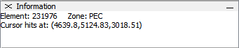
Figure 3.25 Sample “Information” control set