Tutorial 1 - Initial Condition

Disclaimer: The following tutorials are for training purposes only. The three tutorials provided are not designed to simulate real conditions or actual mine-dewatering systems. The problem descriptions are provided solely for the purpose of training a user to use the features of MINEDW and should not be assumed to be representative of actual groundwater modeling methodology or real-world problems. Professional judgment and experience are required to set up a well-defined groundwater flow model to produce meaningful results.

The following examples are prepared for new users of MINEDW. They provide information on the capabilities and functions of MINEDW as well as explain the step-by-step procedure for setting up a MINEDW model.

These tutorials do not cover detailed operations of each MINEDW feature; users should refer to the User Manual for detailed explanations.

General Procedures for Model Construction and Simulation

A steady-state simulation includes the following steps:

• Constructing a mesh using a two-dimensional (2-D) Mesh Generator. (Note: The Mesh Generator is a third-party program, Rhinoceros). The 2-D mesh needs to be saved and then imported into the MINEDW graphical user interface (GUI) to create a three-dimensional (3-D) mesh.

• Assigning additional layers using the “pinch-out” method.

• Defining project properties, such as units (meters or feet), type of simulation (i.e., steady state), closure criteria, solver type, and solver parameters.

• Importing the 2-D mesh and adding layers for the 3-D mesh.

• Adding topographic information for land surface and geology.

• Defining hydraulic conductivity zone properties and then assigning the zones to elements.

• Assigning boundary conditions, which may include constant heads, drains, rivers, recharge, or evaporation.

Transient model runs include additional steps such as the following:

• Assigning initial conditions from a steady-state simulation.

• Creating a mine plan for open-pit/underground mine(s).

• Defining a zone of relaxation (ZOR) around the open pit or underground excavation, if needed.

• Defining a pit lake if pit-lake formation will be considered.

• Defining pumping wells, pumping rates, and other mining-related structures, such as drain notes.

• Assigning boundary conditions, which may include variable fluxes, constant heads, drains, rivers, evaporation, or recharge.

1.1 Problem Description

Tutorial 1 simulates groundwater flow prior to mining under steady-state conditions. The finite-element mesh for the model is constructed so that the model boundary is well beyond the area that will be affected by drawdown. The model domain is approximately 10,000 meters (m) by 10,000 m and has an average thickness of 1,470 m. The surface topography is incorporated in the model with an elevation range of approximately 800–1,858 meters above mean sea level (mamsl). The grid consists of approximately 136,000 nodes and 260,000 elements within 19 main element layers. The number of elements and nodes will vary depending on how the mesh is constructed in the mesh generator and how many layers and pinch-outs are added in MINEDW. Finer discretization is used to resolve geology, geologic structures, rivers, and mining in the model domain. The simulated geology includes nine hydrogeologic units (overburden, alluvium, weathered bedrock, sandstone, granite, kimberlite, and two faults). The hydraulic parameters of the model were assigned as shown in Table 1.1.

Table 1.1. Hydraulic Parameters Simulated in the Groundwater Flow Model

Properties	Kx	Ky	Kz	Ss	Sy
Overburden	0.1	0.1	0.1	5e-06	0.005
Alluvium	0.6	0.6	0.6	5e-06	0.005
Weathered Bedrock	0.0009	0.0009	0.0009	5e-06	0.005
Sandstone	0.00125	0.00125	0.00125	5e-06	0.005
Granite	0.0005	0.0005	0.0005	5e-06	0.005
Kimberlite	0.0005	0.0005	0.0005	5e-06	0.005
Fault-1	0.002	0.002	0.002	5e-06	0.005
Fault-2	0.0002	0.0002	0.0002	5e-06	0.005
Contact	0.003	0.003	0.003	5e-06	0.005

1.2 MINEDW Model Construction

Step 1. Generating a Mesh

It is important to note that the finite-element mesh is constructed using a third-party program, Rhinoceros (Rhino). In order to follow the steps in this tutorial for constructing a model mesh, Rhino must be installed. Additionally, Grasshopper, an algorithmic modeling tool for Rhino, must be installed if Rhino Version 5.0 is used (Grasshopper comes pre-installed in newer versions of Rhino). Rhino is used to create a 2-D mesh that can be imported into the MINEDW GUI, where the remaining model setup occurs.

Open Rhino (if using Rhino 5.0, use the 64-bit option), click on the “File” menu, then select “Import,” as shown in Figure 1.1. Using the “Import” dialog box that opens, navigate to the location where the tutorial files are stored, INPUT>MESH_INPUT>DXF, and select “BOUNDARY.dxf,” then click “Open.” Repeat these steps for each of the files in the INPUT>MESH_INPUT>DXF directory. If the imported objects do not appear in the view ports, select the “Zoom Extents” on the “Standard” tool tab. All imported objects should now be visible.

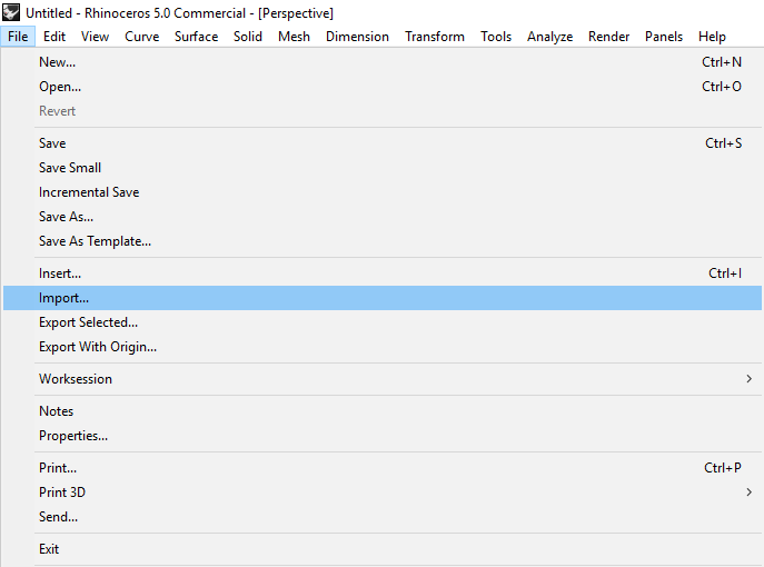
Figure 1.1 The “File” menu

Rhino has four default layout view ports to view the imported data: “Perspective,” “Top,” “Front,” and “Right” (Figure 1.2). Because MINEDW requires a 2-D mesh, all work can be conducted using the “Top” layout. The other layouts are useful for checking that all mesh input items lie within the same plane, as the mesh generator in Rhino requires that all mesh items be within the same plane. Verify that all imported items are within the same plane by using the “Perspective” layout to rotate the imported data in 3-D. To do this, right-click and drag within the layout.

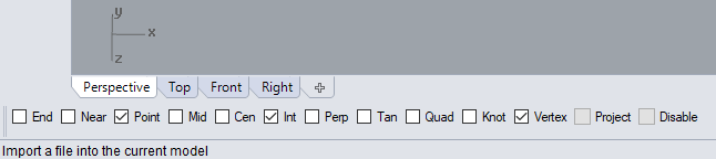
Figure 1.2 The default view ports in Rhino

After importing the required files, the result should appear similar to Figure 1.3. The “MODEL BOUNDARY” must be a completely closed region in order to generate a mesh. The “OPEN PIT” and “TRANSITION ZONE” (Figures 1.3 and 1.4) regions will contain a refined mesh and must be closed as well. The “STREAM NETWORK” represents a series of interconnected streams. The mesh generator will create a mesh that honors the stream network by placing mesh nodes along each stream segment. The “PUMPING WELL” points are the locations of dewatering wells in and around the open pit. The mesh generator will honor these locations by placing a node at each one of the points. Adding additional wells to an existing MINEDW model is done within MINEDW and does not require the mesh to be re-created. For existing models, the user can move the closest mesh node to the location of the pump that is being added.

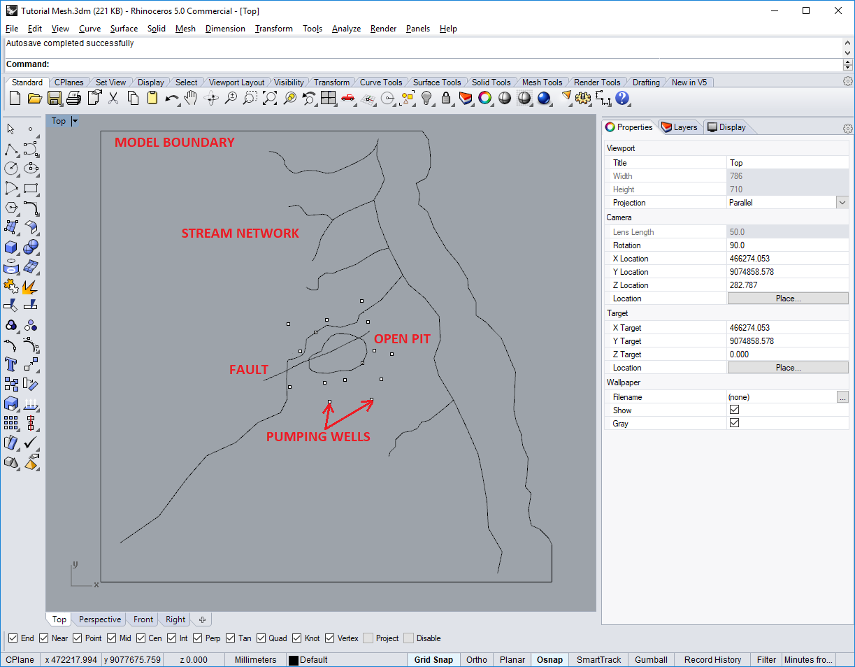
Figure 1.3 The overlay data used to create a mesh

To create the transition zone, click on the “Polyline” tool on the “Standard” tab (Figure 1.4). Next, draw a circle around the “OPEN PIT” object. To finish and close the transition zone, click on the first point of the circle; the drawing tool will likely snap to this point once the mouse pointer gets close enough. The completed transition zone should appear similar to the one shown in Figure 1.4.

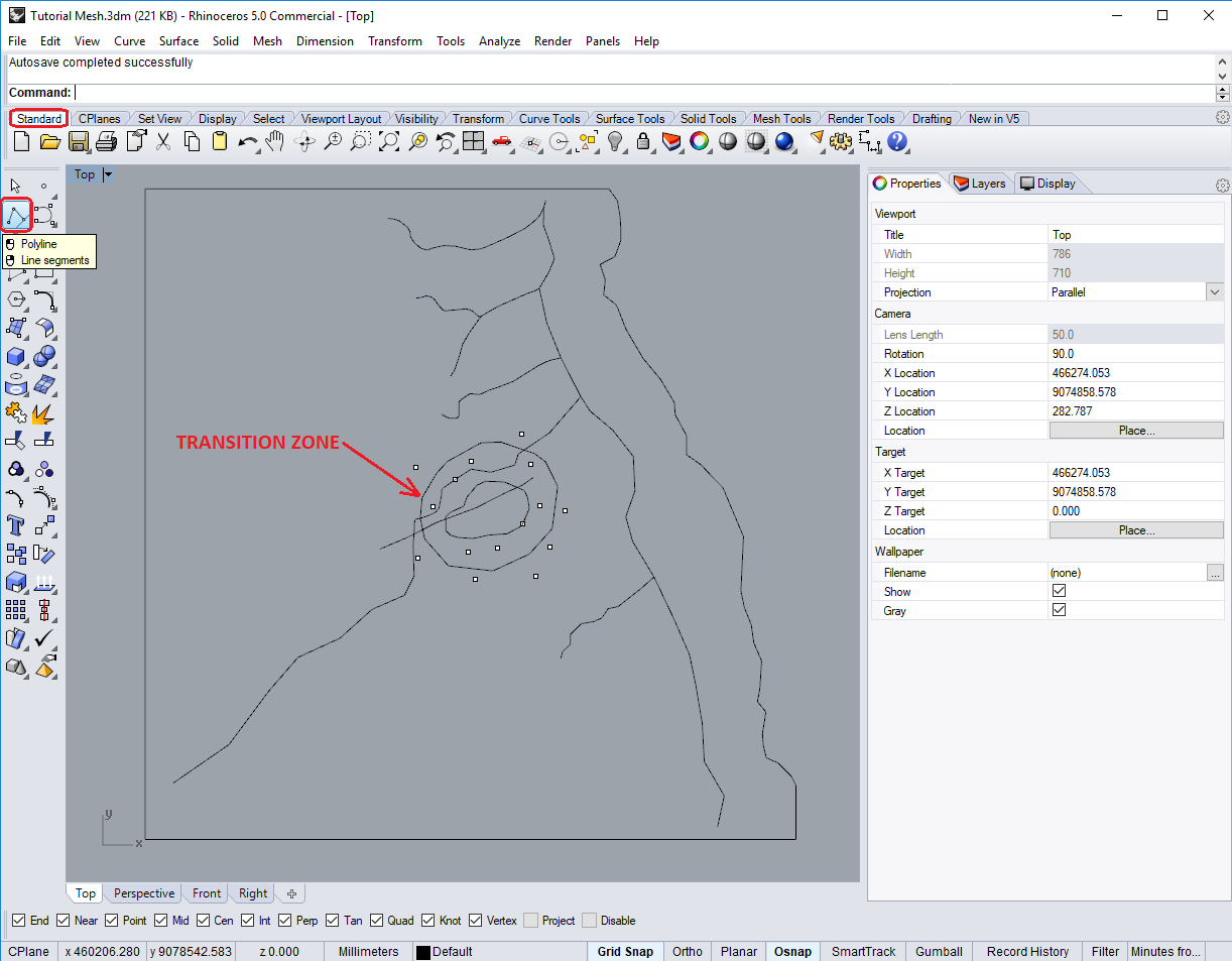
Figure 1.4 The completed transition zone

After completing the transition zone, open Grasshopper by typing “grasshopper” into the command line and pressing [ENTER]. A new window will open for Grasshopper. If you are using Rhino 5 and Grasshopper is not installed yet, download and install Grasshopper for Rhino. Grasshopper does not require an additional license or fee. In Grasshopper, select “File>New Document” to create a new mesh algorithm. Next, click the “MMesh” tab. The “MMesh Util” contains three components, “Fault,” “Region,” and “MMesh.” To create the finite-element mesh for this tutorial, one (1) “Fault” component, three (3) “Region” components, and one (1) “MMesh” component will be needed. Place these components on the canvas by clicking on them in the banner menu and then clicking on the canvas. Each component can be moved around on the canvas as necessary by clicking and holding then dragging the component to the desired location. Each component can be renamed by right-clicking on it and then entering a new name where the component’s current name appears.

In order to complete the mesh, additional components are needed: one (1) “Panel,” five (5) “Number Sliders,” one (1) “Boolean Toggle,” one (1) “Curve,” one (1) “Point,” and one (1) “Merge.” All of these components, except for the “Merge” component, can be found on the “Params” tab under the “Geometry” or “Input” groups (Figure 1.5).

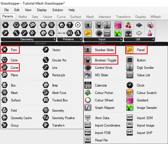
Figure 1.5 Grasshopper components used to create the finite-element mesh

The “Merge” component is used to merge generic streams of data. For example, it is used in this tutorial demonstration to merge the three regions (“MODEL BOUNDARY,” “TRANSITION ZONE,” and “OPEN PIT”) into one data stream for processing. This component is found on the “Sets” tab under the “Tree” group (Figure 1.6).

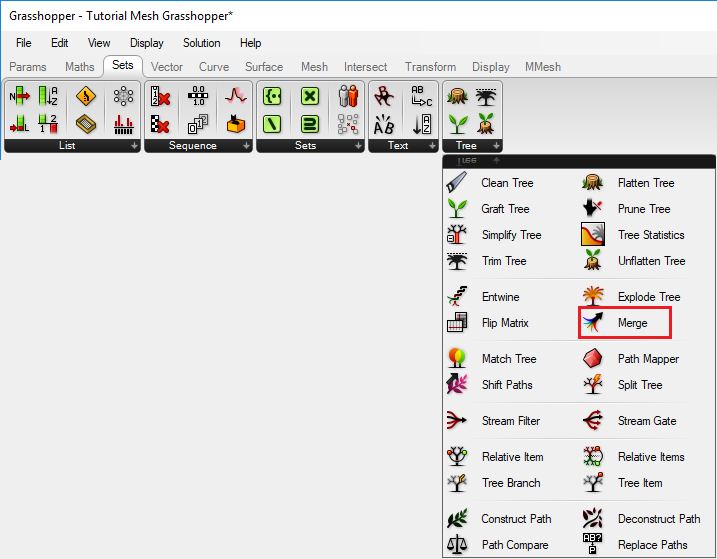
Figure 1.6 The “Merge” component in Grasshopper

After adding all of the necessary components to the canvas, connect them together following the example in Figure 1.7. The easiest method for connecting components is to click on the half circles that appear to the left or right of the component parameter and drag them to the appropriate component. Figure 1.7 can be used as an example of how to arrange and connect the various components.

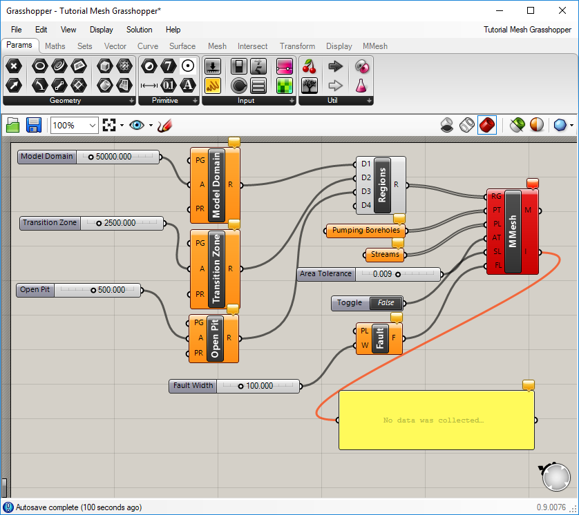
Figure 1.7 Connected Grasshopper components and parameters

Once the components are properly connected, it is time to define parameters for each component. For each number slider, add a name and define the range. In this tutorial demonstration, the number sliders have been named “Model Domain,” “Transition Zone,” “Open Pit,” “Area Tolerance,” and “Fault Width.” The ranges for these number sliders are the following, respectively: 25,000–250,000, 1,000–10,000, 100–1,000, 0.001–0.1, and 25–250. To define the initial value, specify the ranges, and name the number sliders, right-click on each number slider and select “Edit” in the drop-down list. In the “Slider” window, you can enter a “Name” and specify the “Min” and “Max” and set the current value. After completing the changes, click “OK” to save the changes and close the “Slider” window. The other components can be renamed by right-clicking on the component and entering a new name where the current name appears in the drop-down menu. At this point, it may be advisable to save the Grasshopper document so as not to lose any work should anything happen.

After saving the Grasshopper document, assign the “Polygon (PG)” and “Primary Region (PR)” parameters for the “Region” components. Note that the “Area (A)” parameters are defined by connecting the parameters to the number sliders. The “MODEL DOMAIN” curve will be assigned to the “PG” parameter of the “Model Domain” component, the “TRANSITION ZONE” curve will be assigned to the “Transition Zone,” and the “OPEN PIT” curve will be assigned to the “Open Pit” component. To assign a component to a curve, right-click on “PG” and then select “Set One Curve” from the drop-down menu. The Grasshopper window will disappear to show the Rhino window. In the Rhino window, click on the appropriate curve and the Grasshopper window will reappear. Repeat these steps for the other regions.

By default, the “Primary Region (PR)” parameter will be assigned “False” for each of the “Region” components. For the “Model Domain” component, this will need to be changed, and the “PR” component will need to be assigned “True.” To do this, right-click on the “PR” parameter of the “Model Domain” component and then select “Set Boolean>True” from the drop-down list. This parameter identifies the outermost boundary of the mesh to be created. As many regions as needed can be added to the mesh, but only one can be the primary region and must include (surround) all of the other regions.

To assign the fault, repeat the previously described steps, but instead of a “PG” parameter, “PL” is the parameter that will need to be set. The “Streams” component needs to be assigned to the “STREAM NETWORK” in the Rhino window. This assignment is done the same way as the other assignments previously described, but instead of selecting “Set One Curve,” click on “Set Multiple Curves.” Using this option, you can select all of the curves that represent the streams in the Rhino window. After selecting all of the curves, simply press [ENTER] to finish the assignment. The final component that needs to be assigned is the “Pumping Borehole,” which requires points. Follow the same steps as previously described for the other components and select “Set Multiple Points.” In the Rhino window, you can select each point representing the pumping boreholes by hand as you did with the streams, or you can use a Rhino function to do it all at once. To use the Rhino function, type “selpt” into the command line and press [ENTER]. Rhino will select the points and print out how many points were selected, in this case 15 points. After completing the selection, press [ENTER] again to complete the assignment.

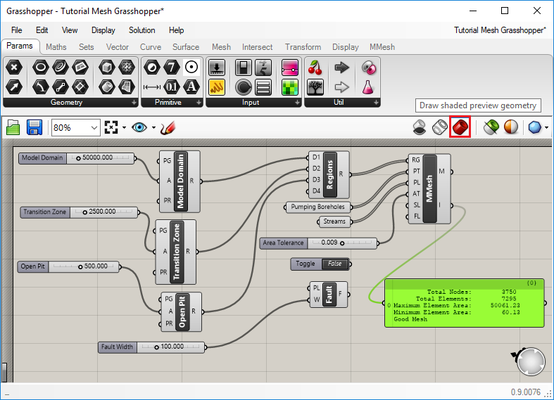
Figure 1.8 The output from the Grasshopper algorithm

Once properly configured, the Grasshopper algorithm will generate a mesh that is visible in the Rhino window. If it is not visible, be sure to toggle the “Draw shaded preview geometry” as shown in Figure 1.8. If the mesh still does not display, check that “Preview Mesh Edges” is turned on by selecting it under the “Display” menu or pressing the [Ctrl] and [M] keys together. The “Panel” item that was connected to the “MMesh” region will display details about the mesh, such as the number of nodes and elements and the minimum and maximum size of the elements. Figure 1.9 is an example of what the mesh created by the Grasshopper algorithm should look like. Note, if you close the Grasshopper window, this mesh will disappear, but as long as you have saved the changes to the Grasshopper document, opening the Grasshopper document will regenerate this mesh.

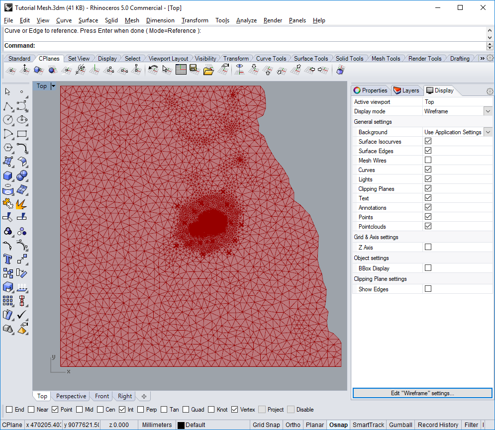
Figure 1.9 The Grasshopper-generated mesh

In order to finalize the mesh and export it in a format that is usable by MINEDW, the Grasshopper-generated mesh needs to be “Bake[d].” To do this, right-click on the “MMesh” component in Grasshopper and select “Bake” from the drop-down menu. An “Attributes” window will open where you can select the layer where you wish to “Bake” the mesh. Any layer is acceptable. The result of this operation should look similar to that in Figure 1.10.

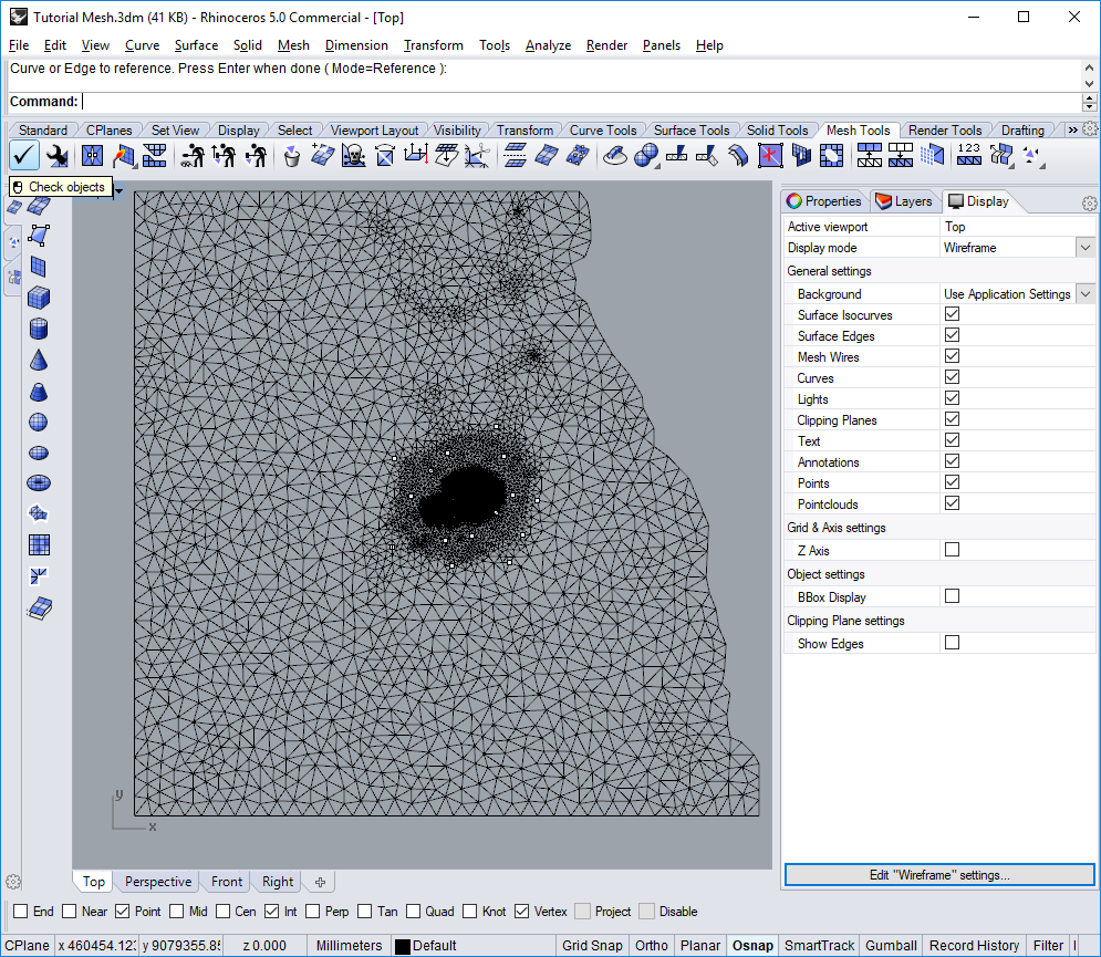
Figure 1.10 The completed mesh in Rhino

After the mesh has been “Bake[d]” to Rhino, it should be checked to ensure there are no problems with the mesh. To check the mesh, click on the “Mesh Tools” tab and then click “Check objects” as shown in Figure 1.10. If there are problems with the mesh, these can be fixed using the mesh tools available in Rhino. Refer to Rhino documentation for instructions on using these functions.

Once the mesh is finished in Rhino, it needs to be exported as an .STL file for import into MINEDW. Select the mesh in Rhino by clicking on it, then select “File>Export Selected…” Using the “Export” dialog box, navigate to where you wish to save the mesh file, then enter a name and select “STL (Stereolithography)(*.stl)” from the “Save as type” drop-down box and click “Save.” Next, in the “STL Export Options,” select the option to export the .STL file in ASCII format, then click “OK.”

1.3 Building the model in MINEDW

Now that the mesh has been created, the mesh is ready to be imported into MINEDW. Open a new MINEDW window and click “File” on the Main Menu banner, and then select “Import.” The “Import File” dialog box appears (Figure 1.11). Select “STL (Stereolithograph) Ascii Files (*.STL)” from the list of options under the “Files of Type” drop-down list. Navigate to the location where you created the mesh file, select it, and click “Open.” IMPORTANT: No mesh will appear in MINEDW at this time; a few more steps must be taken before the mesh is displayed.

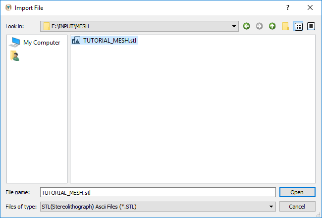
Figure 1.11 The “Import File” dialog box

After importing the mesh, save the MINEDW project file. Select “File”>“Save as” and, using the “Create a MINEDW Project File” dialog box that opens, navigate to the location where you wish to save the model files. In the “File Name” box, enter the name of the project, for example, “SS-TUTORIAL,” and then click on “Save” to create the project file and close the dialog box.

Step 2. Defining Project Properties

To define the project properties such as units (meters or feet), type of simulation, closure criteria, and type of solver, click “Project” and then select “Project Properties.” The “Project Properties” dialog box shown in Figure 1.9 appears. Make sure that all the fields contain the values shown in Figure 1.12. For steady-state simulations, the “Steady State” option should be selected.

For this simulation, the SAMG solver will be used. The outer closure criterion is based on head, while the inner closure criterion is based on mass. Because of this, the inner closure criterion needs be less than 1 x 10^-10, while the outer closure criterion is likely to be greater than 1 x 10^-3. Differences in the closure criterion selection will affect the residual error in the model. Users should check the budget (.BUD) and output (.OUT) files to evaluate the accuracy of the model run and whether more stringent closure criteria are necessary. Maximum inner iterations should be large (i.e., greater than 250); however, the user can evaluate the optimal amount by consulting the MINEDW output file.

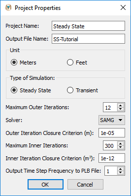
Figure 1.12 The “Project Properties” dialog box

Step 3. Defining Time Steps

To define the time steps for the project, click “Project” on the Main Menu banner, then select “Time Steps.” The “Setup Time Step” dialog box (Figure 1.13) appears. Set the “Maximum # of Time Steps” to 100 or greater. Enter “31” for the “Initial Time Step Length.” For steady-state simulations, only the length of the first time step will be used. Each subsequent time step will be 1.2 times longer than the previous time step. For transient simulations, the multiplication factor is 1 and the time-step length is defined in the “Setup Time Step” dialog box for transient model runs. Ensure that the “# of Time Steps for This Simulation” slider is set to 100 or greater and that the “Start at Time Step” combo box is set to 1. Click “OK” to save the changes and close the “Setup Time Step” dialog box.

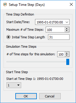
Figure 1.13 The “Setup Time Step” dialog box

Step 4. Importing Ground-Surface Elevation

To incorporate the ground-surface elevation in the model, select the “List” tab in the “Control Panel” pane on the right-hand side of the MINEDW interface. Expand the “Node” item by double-clicking the “Node” item or clicking on the small triangle next to “Node.” Next, double-click “2D Contour” as shown in Figure 1.14. The mesh will be displayed in the plot pane.

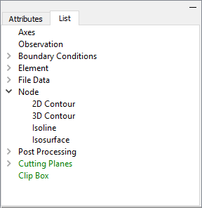
Figure 1.14 The “Control Panel” with activated “List” tab and “Node” plot item

From the “Control Panel” pane on the right-hand side of the MINEDW interface, select the “Attributes” tab. Make sure that the “Color By” attribute is set to “Elevation” and that the “Layer” attribute is set to 1 (Figure 1.15). Next, click the “Select” tool on the Main Menu banner.

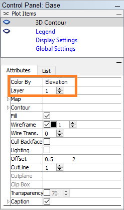
Figure 1.15 The “Control Panel” pane showing the “Attributes” tab with “Layer” set to “1”

In the MINEDW View Pane, use the cursor to click and drag a box around the whole domain to select all of the nodes in Layer 1. Press the [Enter] key to open the “Assign Properties for Nodes” dialog box shown in Figure 1.16. Click “Interpolate From File” and the “Open Data File” dialog box appears. Select the data file in the directory “/INPUT/SURFACE” named “SURFACEELEV.DAT” and click “Open.” The “Grid” dialog box shown in Figure 1.17 appears. Define the interpolation method (Inverse Distance or Kriging) and the required parameters and then click “OK.” The interpolation procedure assigns the ground-surface elevation contained in the “SURFACEELEV.DAT” file to the first layer of the model.

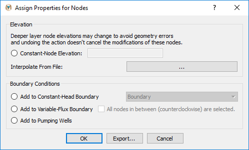
Figure 1.16 The “Assign Properties for Nodes” operations dialog box

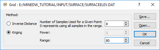
Figure 1.17 The “Grid” dialog box and example values for surface interpolation

View the ground-surface elevation as contours by clicking on the “Attributes” tab in the “Control Panel” pane. Next, click on the small triangle next to “Contour.” Deselect the “Auto” box next to “Minimum” and replace the default value with 800. You may also wish to change the contour interval; smaller numbers produce a smoother color flood. Press [Enter] and the model will appear similar to what is displayed in Figure 1.18.

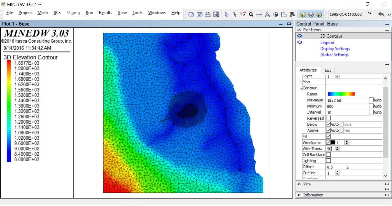
Figure 1.18 MINEDW color flood of topography

Step 5. Adding Layers

To add layers, select “Mesh” from the Main Menu banner, then select “Define Main Layer.” The “Define Main Nodal Layers” dialog box (Figure 1.19) appears. Select the bottom layer. To add a node layer above the selected node layer, click “Insert.” For this model, three layers will be created using the “Depth” method with thicknesses of 20, 30, and 50 m (Figure 1.20). Next, add three more layers but choose the “Average” method. Finally, add 11 more layers for a total of 19 layers and choose “Constant” from the “Method” drop-down box (Figure 1.20). For the layers with the “Constant” method selected, enter the values displayed in Figure 1.20. Note: Do not change the elevation of the first node layer because its elevation was assigned by interpolation. Once you have finished entering the required information, click “OK” to add the layers. MINEDW will produce a warning stating that the ZOR may need to be updated. Disregard this message, as no ZOR has been defined. For more information on adding layers, refer to the User Manual section 7.2.2.

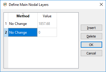
Figure 1.19 The “Define Main Nodal Layers” dialog box

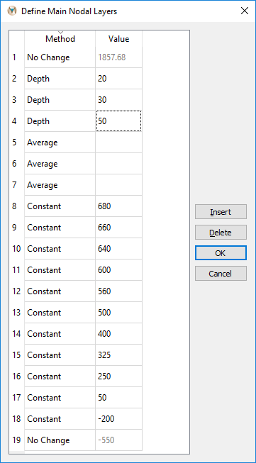
Figure 1.20 The “Define Main Nodal Layers” dialog box showing different methods available

Step 6. Defining Zone Properties

To define the properties of a hydraulic zone, click “Project” on the Main Menu banner and then select “Zone Properties.” The “Zone Properties” dialog box (Figure 1.21) appears. To add a new zone, click the “Add” button. Enter the zones and related hydraulic properties as listed in Figure 1.21 and then click “OK.”

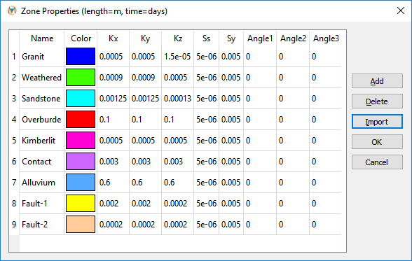
Figure 1.21 The “Zone Properties” dialog box

Step 7. Assigning Hydraulic Zones to Elements

From the MINEDW main window, select the “List” tab in the “Control Panel” pane. Expand the “Element” item and double-click “3D Element,” as shown in Figure 1.22. While working on element-related operations, such as assigning hydraulic zones, ensure that all other plot items related to “Node,” such as a “Contour” plot, are deactivated or deleted from the View Pane (MINEDW Manual 3.4.1).

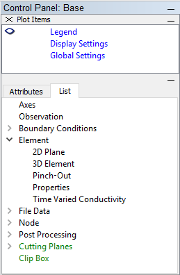
Figure 1.22 The “Control Panel” with the “List” tab and “Element” plot item activated

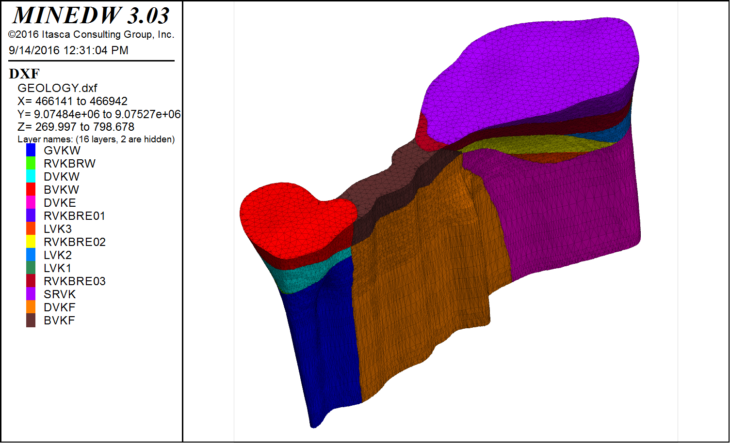
Figure 1.23 A wireframe format of a geological block model

In MINEDW, the assignment of hydraulic zones can be done using a 3-D .DXF with a wireframe format of a geological block model (Figure 1.23). In this tutorial, hydraulic zones will be assigned in two steps. First, regional geology will be assigned by layers and then a kimberlite and a contact zone will be assigned using a 3-D wireframe .DXF file. The regional geology consists of overburden, weathered bedrock, sandstone, and granite. To assign the regional hydraulic zones, click the “Select” tool. Make sure that “Layer” under the “Attributes” tab shown in Figure 1.24 under the “Control Panel” pane is set to 1.

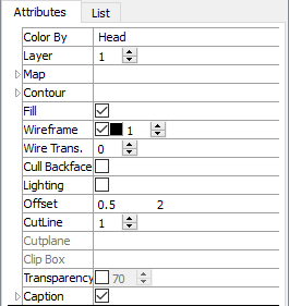
Figure 1.24 The “Attributes” tab with “Layer” set to 1

Select all the elements on the first layer by using the cursor to click and drag a selection box as shown in Figure 1.25, then press the [Enter] key.

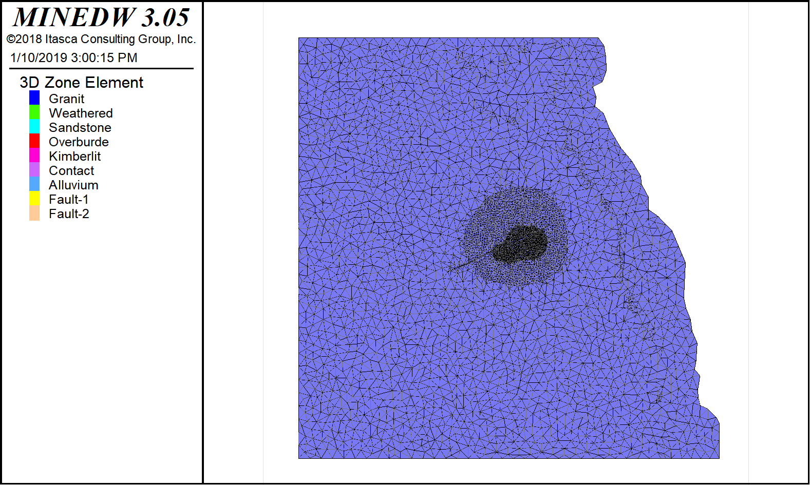
Figure 1.25 Selection of first layer of elements

The “Select Geological Zone:” dialog box shown in Figure 1.26 appears. Change the “Zone” to “Overburden,” change the value in the box next to “From Current Layer #1 To” from 1 to 2, and then click “OK.”

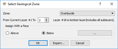
Figure 1.26 The “Select Geological Zone:” operations dialog box

To assign the weathered unit, change the value for the “Layer” attribute on the “Attributes” tab to 3. Select all the elements on the third layer by using the cursor to click and drag a selection box, then press the [Enter] key. The “Select Geological Zone:” operations dialog box appears. Change the “Zone” to “Weathered,” leave the value in the box next to “From Current Layer #3 To” as 3, and then click “OK”.

The “Sandstone” unit is below the “Weathered” unit. To assign it to the model, click the “Select” button. Make sure that the “Layer” attribute on the “Attributes” tab under the “Control Panel” is set to 4. Select all the elements in the fourth layer by using the cursor to click and drag a selection box and then press the [Enter] key. The “Select Geological Zone:” operations dialog box appears. Change the “Zone” to “Sandstone” and the value in the “From Current Layer #4 To” box to 6 and then click “OK.” Finally, assign “Granite” using the same steps as above, from “Layer 7” to “Layer 18,” if it has not already been done.

This model also includes an alluvial zone in a river channel, two fault zones, and a contact zone between the kimberlite pipe and surrounding geology. The alluvial zone representing the river channel can be selected using an ESRI shapefile. The shapefile was created by using the buffer tool in ArcMap and the River.BLN files used in the Mesh Generator. To select elements in the river channel, click the “List” tab and then click the arrow next to “File Data.” Double-click “ESRI Shape File” and then on the “Attributes” tab click the plus sign. Browse to the “STREAM_ALLUVIUM.SHP” file and select it, then click “Open.” If you do not see the polygon buffer representing the river, ensure the “Project to Surface” box is checked. Make sure that “Layer” under the “Attributes” tab under the “Control Panel” pane is set to 1.

Next, click the “Select With Overlay” tool and click the “Polygon” radio button, then click “OK.” The elements that form the river channel should now be selected; press [Enter]. Change the “Zone” combo box to “Alluvium” and change the “To Layer” value to 3 (Figure 1.27), then click “OK.”

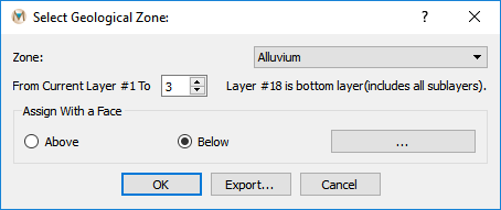
Figure 1.27 The “Select Geological Zone” dialog box

To assign the “Kimberlite” and “Contact” zones using a 3-D .DXF, add a “DXF” plot item from the “Control Panel” pane by choosing “List” then “File Data.” Expand “File Data” by clicking on the small triangle next to “File Data.” Under “File Data,” double-click on “DXF.” The “Attributes” tab will appear (Figure 1.28). Click on the “+” next to “File.” The “Select DXF data file” window will appear. Select the “GEOLOGY.DXF” file. All of the geologic units are present in this 3-D .DXF file. In order to view just the geologic units of interest, select the “Attributes” tab, then click the triangle next to “Layers.” Uncheck the boxes next to “OVB” and “GNS.” The remaining geologic units will be used to represent the contact zone and the kimberlite pipe.

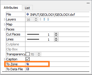
Figure 1.28 The “Attributes” tab

To define the contact zone, click on the “To Zone” button (Figure 1.28) and then select “Contact” from the combo box (Figure 1.29). Then check “Face” in the box next to “Layer Thickness,” enter 20, then click “OK.” The process may take some time, but the area will be assigned to the contact zone. Note: The contact zone may need to be adjusted manually by selecting elements with the “Select” tool. To assign elements with “Kimberlite” properties, repeat the steps above but select “Kimberlite” instead of “Contact” and check “Volume” and “Whole.” The volume representing the kimberlite pipe will need to be adjusted manually by adjusting element properties individually; see Figure 1.30 for a reference of what the final kimberlite and contact zones look like.

Figure 1.30 shows the two fault zones that intersect the kimberlite pipe. The fault zones are assigned using the “Select with Overlay” tool. To do this, click on the “List” tab in the “Control Panel” pane, click “File Data,” and then double-click “BLN.” Next, click on the button next to “File” on the “Attributes” tab and navigate to the “FAULT.BLN” file. The “FAULT.BLN” should be projected to the surface automatically, making it visible. If it is not visible when opened, check the “Project to Surface” box on the attributes tab. If the “RIVER.SHP” file is still visible in the View Pane or “Plot Items” pane, remove it before proceeding. Make sure that “Layer” under the “Attributes” tab under the “Control Panel” pane is set to 1. Next, click on the “Select” tool if it is not already selected and click the “Select with Overlay” button. Then check the button next to “Polyline” and click “OK.” Fault-zone elements should now be selected. Press the [Enter] key to bring up the “Select Geological Zone:” dialog box. In the box next to “From Current Layer #1 to,” enter “18,” which is the bottom, and select “Fault 1,” then click “OK.” The section of the fault that intersects the contact and kimberlite zones will need to be selected by hand and assigned to “Fault 2” (Figure 1.30).

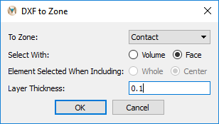
Figure 1.29 The “DXF to Zone” dialog box

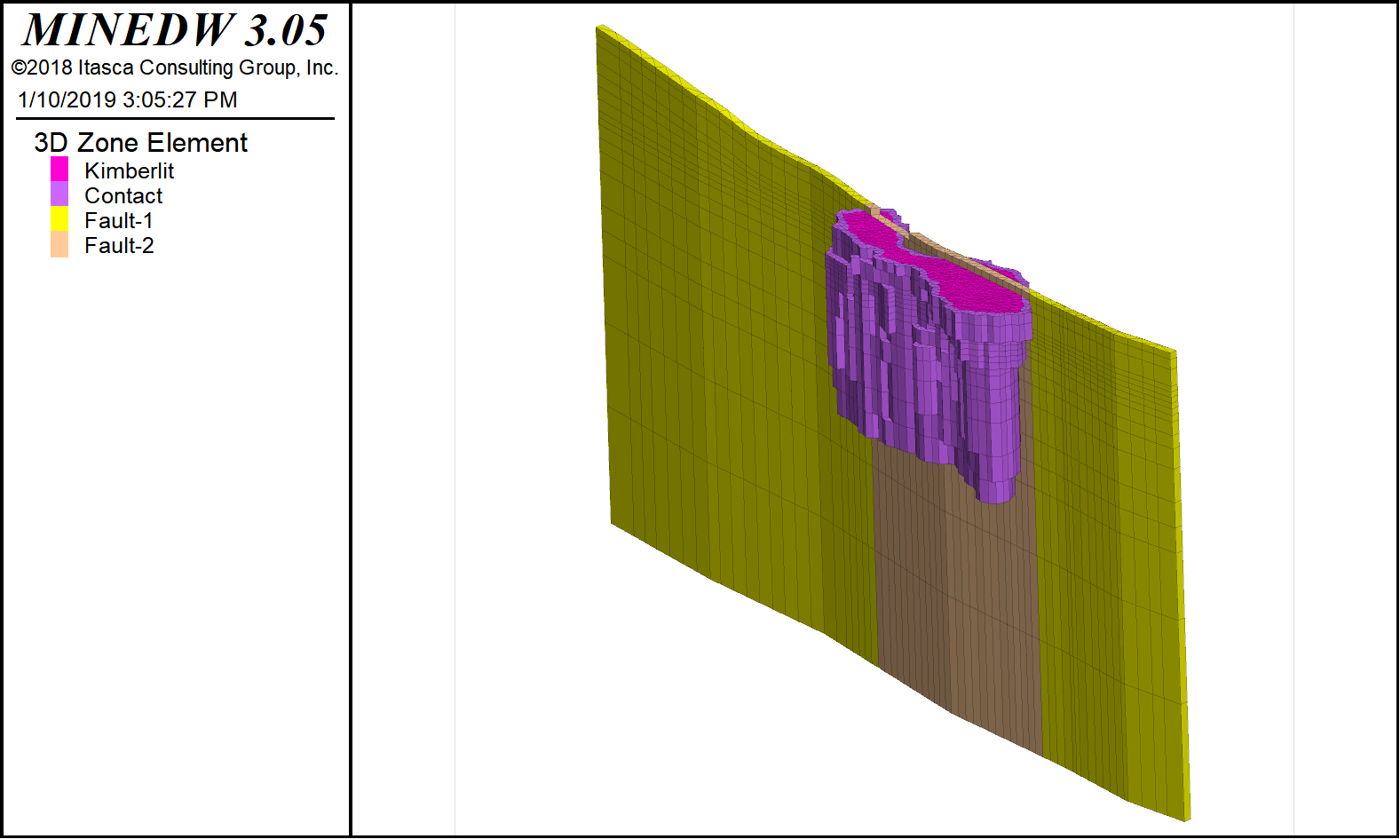
Figure 1.30 The completed contact zone, kimberlite pipe, and fault zones

For a detailed explanation of how to cut cross sections, please refer to the MINEDW User Manual section 9.12. Briefly, to create a cross section, add a “3D Element” plot item to the View Pane, then select the “Create Plane…” tool on the menu banner. Select two points on the “3D Element” plot item, and the cross section will appear. Rotate the cross section manually or click the “Snap View” button on the “Attributes” tab of the “Plane” plot item to better orient the cross section. To create a cross section similar to the one displayed in Figure 1.31, click on the “3D Element” plot item, then select its “Attributes” tab and locate the “Cutplane” attribute. Check the boxes next to “On” and “Front.”

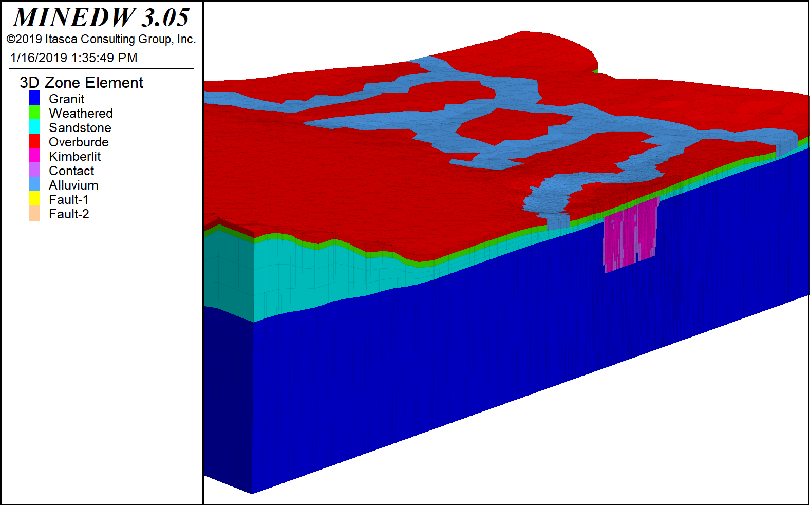
Figure 1.31 Cross section of the geological units in the model

Step 8. Defining “Pinch-Outs”

MINEDW is able to simulate locally refined vertical discretization in areas of interest. The enhanced discretization is referred to as a pinch-out since layers pinch out where the vertical discretization is not needed. Defining pinch-outs in the steady-state model is necessary because hydraulic heads from the steady-state model will be used as initial conditions for the transient model run, which requires that both models have identical meshes. To define the pinch-out types, select “Mesh” from the Main Menu banner and then select “Define Pinch-Out…” The “Define Pinch-Outs” dialog box appears (Figure 1.32).

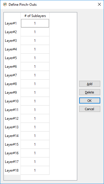
Figure 1.32 The “Define Pinch-Outs” dialog box

In MINEDW, various pinch-out configurations can be defined and simulated. Each configuration is defined as one type of pinch-out. Based on modeling needs, the user can define as many pinch-out configurations as necessary.

Figure 1.33 illustrates the working principle of the pinch-out method. For example, suppose a model has four regional layers that are each represented (sequentially, Layer 1 to Layer 4, from top to bottom) by a black square. The column labeled “# of Layer after Pinch-out” shows the number of pinch-out layers (shown in blue) allowed for each model layer. For illustration purposes, pinch-outs have been created in two layers, and using these pinch-outs, three different pinch-out types have been created (Figure 1.33). Type 1 consists of three pinch-outs in model Layer 2 (depicted by red lines). Type 2 consists of three pinch-outs in model Layer 2 and two pinch-outs in model Layer 3 (depicted by a green line). Type 3 consists of two pinch-outs in model Layer 3. When assigning pinch-outs to the elements, only one type can be assigned to a selected location. It should be noted that, for each model layer, MINEDW only allows one value for the number of pinch-outs (e.g., Layer 3 can only have two pinch-outs. It cannot have two pinch-outs in one area and three pinch-outs in another area).

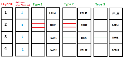
Figure 1.33 Schematic explanation of pinch-outs

To define pinch-outs, click the “Add” button on the right side of the “Define Pinch-Outs” dialog box to add pinch-out types.

In this tutorial model, there is one type of pinch-out. This pinch-out type (“Type 1”) has two pinch-outs in Layers 3 through 15. Type in the number of pinch-outs in the “# of Sublayers” column and create the pinch-out type by checking the box next to the appropriate layer under the “Type #” field (Figure 1.34), then click “OK.”

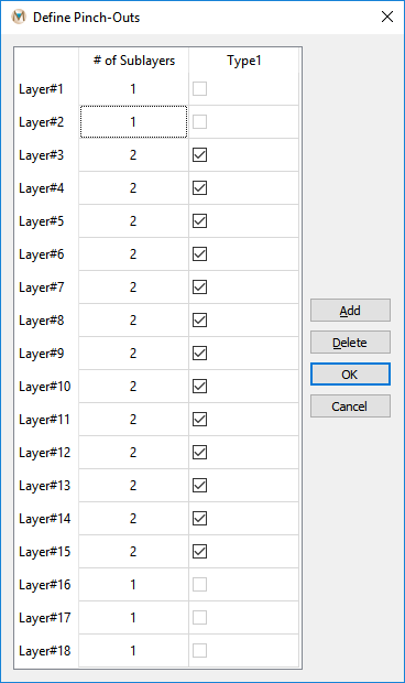
Figure 1.34 The “Define Pinch-Outs” dialog box

To add pinch-outs to a selected area, select the “List” tab in the “Control Panel” pane. Expand the “Element” item, and double-click “Pinch-Out,” as shown in Figure 1.35.

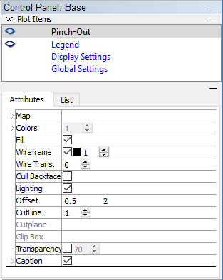
Figure 1.35 The “Pinch-Out” plot item “Attributes”

From the main window, click the “Select” button on the Main Menu banner. Select the nodes that define the elements where the “Type 1” pinch-out will be created by clicking the “Select with Polygon” button and selecting the nodes as shown in Figure 1.36.

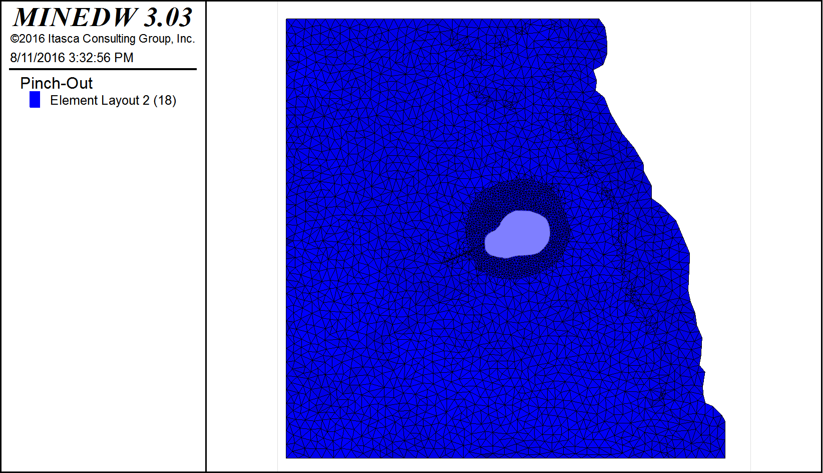
Figure 1.36 The View Pane with the selected nodes for pinch-out Type 1

Press the [Enter] key. The “Select Pinch-Out Type” dialog box appears. Select “Type 1” (Figure 1.37) and click “OK.”

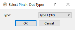
Figure 1.37 The “Select Pinch-Out Type” dialog box showing “Type 1” selected

To view the pinch-out in a cross-section view, delete or turn off the “Pinch-Out” plot item by right-clicking on it and choosing “Delete plot item” or “Deactivate plot item.” Next, add a “3D Element” plot item to the View Pane by clicking the arrow next to “Element” in the “Control Panel” pane and double-clicking on “3D Element.” Next, select the “Create Plane…” tool and select two points on either side of the area where the pinch-out was added. The result should look similar to Figure 1.38.

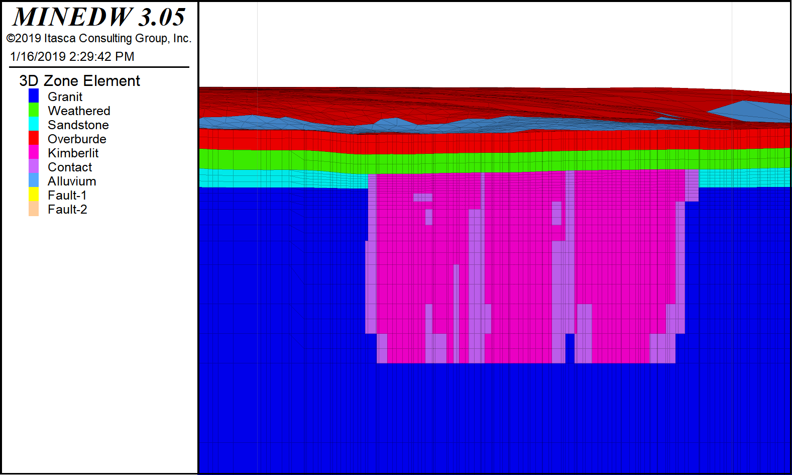
Figure 1.38 The View Pane with the cross-sectional view with pinch-out Type 1

Step 9. Defining Initial Heads

To define the initial heads, click “Project” on the Main Menu banner, then select “Initial Heads.” The “Set Up Initial Head” dialog box appears. Choose “Constant” with a level of 800 m as shown in Figure 1.39.

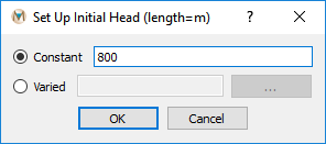
Figure 1.39 The “Set Up Initial Head” dialog box

Step 10. Assigning the Boundary Conditions

To assign boundary conditions, select the “List” tab in the “Control Panel” pane. Expand the “Node” item, and then double-click “3D Contour” (Figure 1.40).

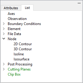
Figure 1.40 The “Control Panel” pane with the “Node” item expanded to show the “3D Contour” option

In this tutorial, three types of boundary conditions are used: constant-head, river, and no-flow boundaries. Assignment of these boundary conditions is discussed in the following sections.

Constant-Head Boundary

In order to add constant-head boundary conditions to the model, begin by defining groups for the constant-head boundary conditions. To do this, select the “Constant Head…” menu item under “BCs” on the Main Menu banner. In the “Constant-Head Boundary” dialog box that opens, click on the “Add” button (at the top of the dialog box) to add a blank group (Figure 1.41). To change the name of the group, click in the drop-down box where the group name appears and change the text (Figure 1.41). Three constant-head groups will be used for this tutorial simulation, “Pond,” “LowLand,” and “MtBlock.” Create these groups as described above and then click “OK” in the “Constant-Head Boundary” dialog box to close the dialog box and save the changes.

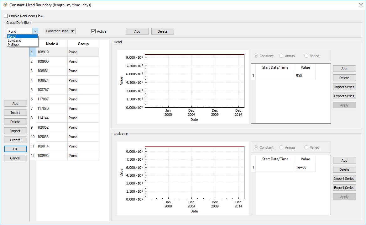
Figure 1.41 The “Define Group for Constant Heads & Drain Nodes” dialog box

To add constant-head boundary conditions to the mesh, select the “3D Contour” plot item from the “Plot Items” list in the “Control Panel” pane. Ensure that the “Layer” attribute under the “Attributes” tab is set to 5, then click the “Select” button on the Main Menu banner. Using the “Select” tool, select the nodes along the southwest perimeter as shown in Figure 1.42 and then press [Enter]. In the “Assign Properties for Nodes” dialog box that appears, select “Add to Constant-Head Boundary” (Figure 1.43). Next, select the “MtBlock” group from the drop-down menu that becomes active and then enter the bottommost layer in the box to the right next to “From Current Layer.” This will assign the constant-head boundary from Layer 5 to the bottom of the model domain.

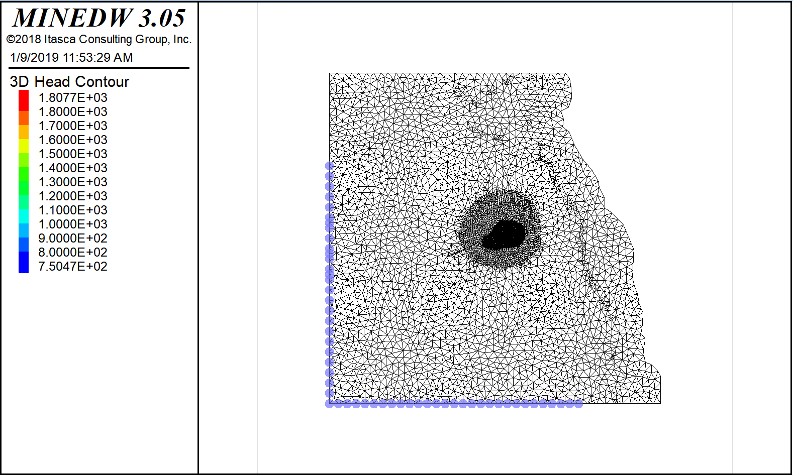
Figure 1.42 The View Pane with the selected constant-head boundary nodes

Repeat the steps described above for the remaining perimeter nodes that have not been assigned a boundary condition. The constant-head boundary group to be used for the remaining nodes that have not been assigned a boundary condition should be “LowLand.” Now that the constant-head nodes have been added to the boundary of the model domain, the constant-head values need to be modified. The default values assigned to the constant-head nodes by MINEDW are the elevations of the nodes. Using these default values would result in a downward hydraulic gradient. The constant-head values for nodes beneath the fifth layer should be the constant-head value of the fifth-layer node directly above. To assign these values, the constant-head value for each of the nodes needs to be recorded then copied to each of the nodes below. This can be done using the “Constant-Head Boundary” dialog box but would be very tedious. The following describes a method to do this using a provided Excel document.

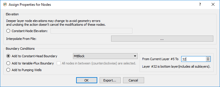
Figure 1.43 The “Assign Properties for Nodes” dialog box

Begin by executing the “Create Data Set” function under the “Run” menu on the Main Menu banner. This function will create several text files in a directory that the user selects. Two of the text files, “chead.dat” and “nodel.fem,” are needed to update the constant-head values. After running the “Create Data Set” function, locate the Excel file named “UpdateCHead.xlsm” in the “INPUT” directory containing the other input files for this tutorial. Copy the file and paste it in the directory where the “Create Data Set” function was executed. Open the Excel document and, if not already active, select the sheet labeled “Input-chead.dat.” Click on the button “Import CHead.dat” to import the chead file that was just created by MINEDW. Using the “Import Text File” dialog box that opens, navigate to the directory where the MINEDW files were created. The files may not be visible in the “Import Text File” dialog box because Excel by default looks for files that have a “.TXT” extension. To view all of the files in the directory through the “Import Text File” dialog box, select “All Files (*.*)” from the drop-down menu on the lower right-hand corner of the dialog box. Now that all of the files that MINEDW created are visible, select the file named “chead.dat,” then click “Open.” Repeat these steps on the “Input-node.FEM” tab, but this time select the file labeled “node.fem.” Now that the input data are imported, create the new constant-head file. Select the “Output-chead.dat” tab and click “Run.” Copy the results from the run function beginning with row 1. Paste the contents into a text editor and save the file as “newChead.dat.” Now that the new chead file has been created, use the “Constant-Head Boundary” dialog box in MINEDW to import the file. Click the “Import” button on the left side of the “Constant-Head Boundary” dialog box and navigate to the location where “newChead.dat” was saved, select it, and click “Open.” The new constant-head values will be imported into the model.

The remaining constant-head group that should be added is the “Pond” group. This group is used to simulate an open-water body located some distance to the northeast of the open pit. Using a “3D Contour” plot item, with the “Layer” attribute set to 1 on the “Attributes” tab, select a few nodes somewhere to the northeast of the pit (Figure 1.45). For this tutorial, it does not matter where the nodes are selected so long as they are not adjacent to the pit. With the nodes selected, press [Enter] to open the “Add Properties for Nodes” dialog box. Click on “Assign to Constant-Head Boundary” and ensure that “Pond” is selected. Leave the “From Current Layer #1 To” as “1” and then click “OK.” The nodes that compose the “Pond” group should all be assigned with the same head value to simulate the water body. To view and edit the assigned constant-head nodes, go to “BCs” on the Main Menu banner and select “Constant Head.”

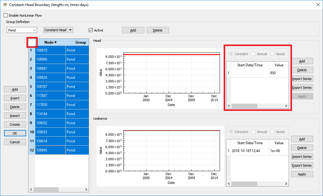
Figure 1.44 The “Constant-Head Boundary” dialog box

Ensure the “Pond” group is the currently selected group in the “Group Definition” drop-down box. Select all of the nodes in the “Pond” constant-head group by clicking in the top left square of the constant-head node box, highlighted in red in Figure 1.44. After selecting the constant-head nodes that will compose the pond feature, change the constant-head value to the desired value, e.g., 950 m. This will update the constant-head value for each of the nodes to 950 m (Figure 1.44). Ensure that the leakance value is also set to a high value to ensure flow to or from the constant-head nodes is not restricted.

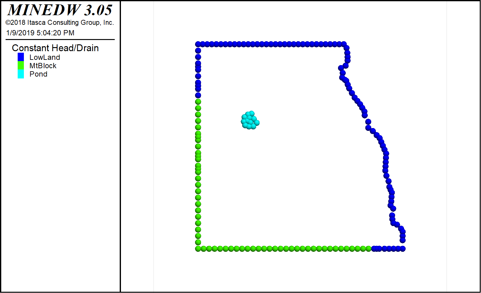
Figure 1.45 The completed constant-head boundary conditions

Figure 1.45 shows the completed constant-head boundary conditions that have been assigned to the model. The “LowLand” and “MtBlock” constant-head values were modified using an Excel document to assign the nodes below the fifth layer a constant-head elevation equal to the elevation of the fifth-layer node directly above. The “Pond” group was used to simulate a body of open water. The constant-head elevation for the “Pond” group was modified in the “Constant-Head Boundary” dialog box.

River Boundary Condition

The “River” boundary condition is used to simulate interactions between a routed river and an aquifer. There are several methods that can be used to add a river boundary condition to a model. This tutorial describes a method using .BLN files to create the river network boundary condition.

To begin, open the “River” dialog box by clicking “BCs” on the Main Menu banner and selecting the “River” menu item. On the “River” tab in the “River” dialog box, click “Add” to add a river segment. Click “Create” in the lower right-hand corner of the “River” tab to open the “Select BLN file” dialog box. Navigate to the directory containing the .BLN files representing the river. These are the same files that were used to create the mesh in Rhino but in individual files for each of the reaches of the river network. Begin by selecting “STREAM_1.BLN” and clicking “Open.” MINEDW will select the appropriate nodes to simulate the river reach and assign a bed elevation at each of the nodes based on the node elevation. The slope of the riverbed will be variable between nodes depending on the nodes’ elevations. Because of this, the “Bed Elev.” of some nodes will need to be adjusted to ensure there is a downward slope from the highest to lowest node. MINEDW will produce a warning if the slope at any of the nodes is incorrect. If a constant riverbed slope is desired, click the “Constant Slope” button to calculate a constant slope for the entire river reach. The slope will be calculated based on the highest and lowest node elevations. Change the default values for the “Manning Coefficient,” “Width,” and “River Bed Thickness” as necessary. The “River” tab is shown in Figure 1.46 with the completed fields.

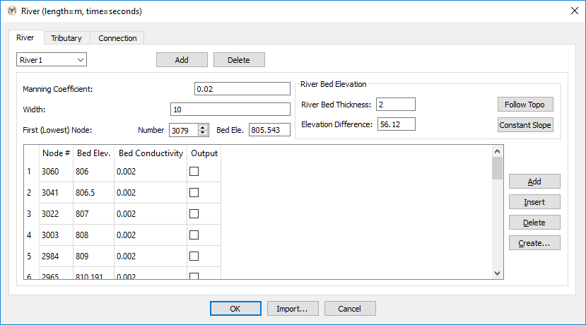
Figure 1.46 Completed river segment 1 and simulation parameters

Repeat the steps above for river reaches 2 through 7. Once all of the river reaches have been created, ensure the connections between reaches are properly defined. To do this, click the “Connection” tab in the “River” dialog box. Click the “Refresh” button at the bottom of the tab. MINEDW will automatically create the connections between connected river reaches. If the bed elevations of the nodes where the river reaches connect do not match, MINEDW will produce a warning indicating where the problem is located. The easiest way to resolve the issue is to adjust the elevation of the upstream reach rather than the downstream reach. Figure 1.47 shows the “Connection” tab with the correctly defined connections for the tutorial.

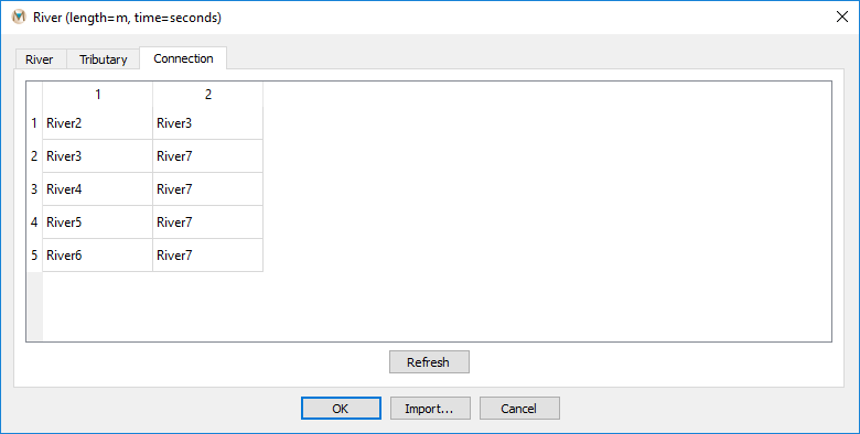
Figure 1.47 The “Connection” tab with connections between river reaches defined

The “Tributary” tab is used to define inflows to river reaches that come from outside of the model domain or from some other external source, such as a pipeline that discharges flow to a river. In this tutorial, two tributaries are simulated, one for River 5 and one for River 7. Although the tributary function can accept temporally varying inputs for a transient simulation, this tutorial will use constant inflow for both the steady-state and transient simulations. Figure 1.48 shows the “Tributary” tab with the tributary for River 5 defined. To correctly define a tributary, it must be on one of the nodes that make up a river reach. In this example, the uppermost node of River 5 was chosen as the tributary node. If a node that is not connected to any river is used, MINEDW will produce a warning indicating that the tributary is not used. If the tributary is correctly defined, the tributary connection to the river will appear on the “Connection” tab when “Refresh” is clicked.

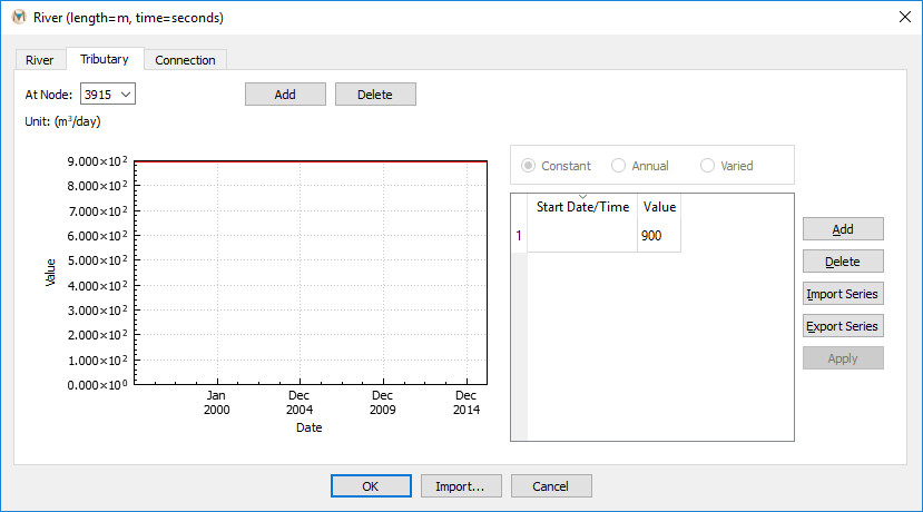
Figure 1.48 The “Tributary” tab showing the tributary for River 5

The completed river boundary condition can be displayed in the view pane by selecting the “River” plot item under the “Boundary Conditions” group in the “Control Panel” pane. Figure 1.49 shows the completed river network and two tributaries that were added to the model.

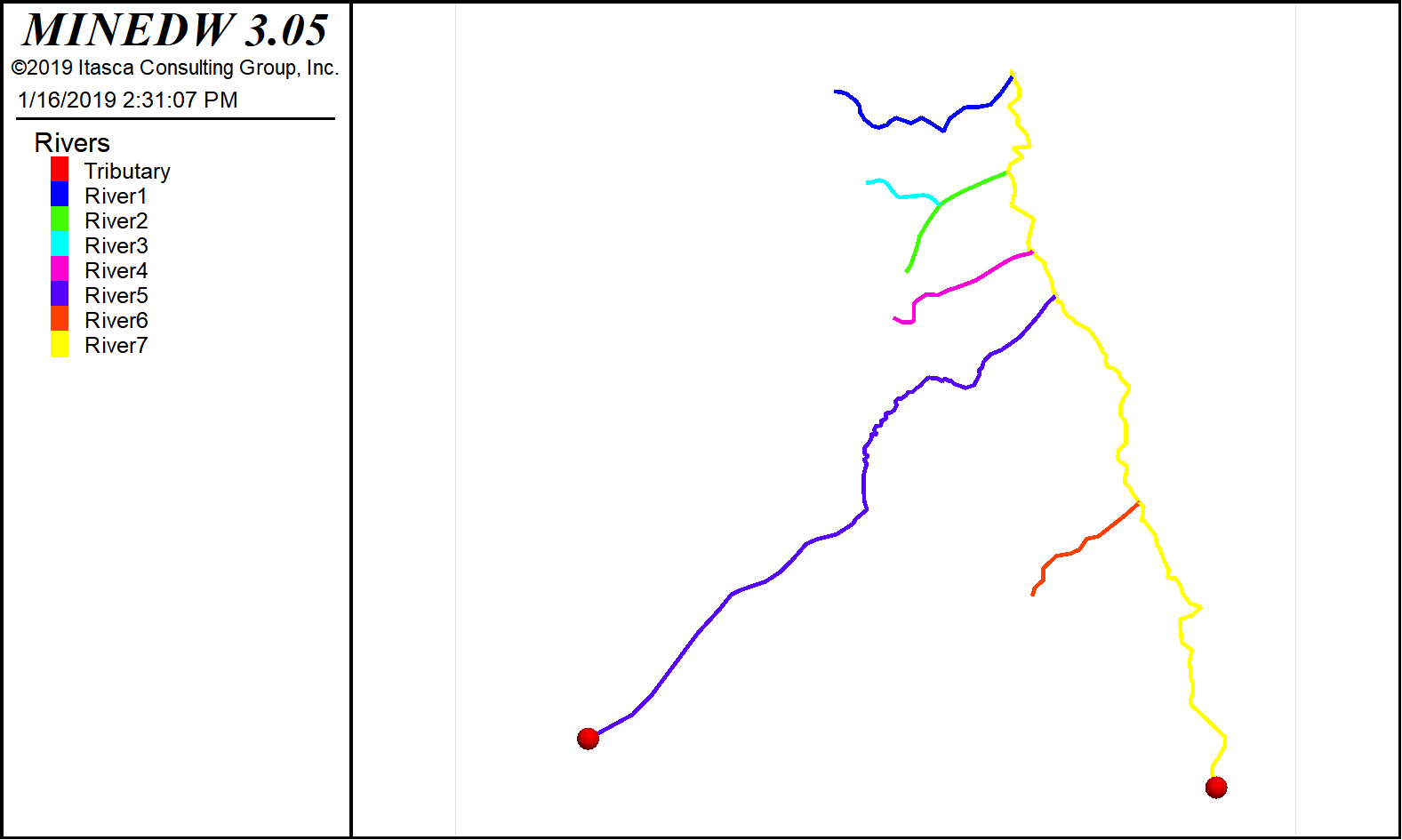
Figure 1.49 The completed river network

No-Flow Boundary

No-flow boundary conditions are assumed by MINEDW for any location along the model domain where other boundary conditions have not been assigned. In this tutorial, the bottom of the model is a no-flow boundary condition.

Step 11. Assigning Recharge

In this tutorial, recharge is applied to the first wet layer of the model. The default option in MINEDW is to apply recharge to the first wet layer, but this can be changed if needed (Figure 1.50). To create recharge zones, click “BCs” on the Main Menu banner, then select “Recharge.” The “Recharge” dialog box (Figure 1.50) appears. Click the “Add Zone” button at the bottom of the dialog box to add a recharge zone. Complete the fields for Zone #1 (Figure 1.50).

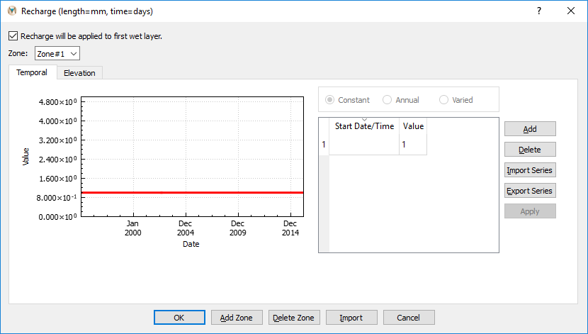
Figure 1.50 The “Recharge” dialog box showing Zone #1

Next, click on the “Elevation” tab and define the parameters for the elevation-based recharge equation (Figure 1.51). This zone will be used to simulate orographically controlled recharge in the model. The parameter values for parameters “A,” “B,” and “C” can be calculated by fitting the equation (Figure 1.51) to a precipitation versus elevation data set. For this tutorial, the parameter values for “A,” “B,” and “C” are provided. The “Factor” that is used is a scaling factor and is explained in further detail in section 7.4.6 of the MINEDW manual.

After entering the parameters required to define the first recharge zone (Figures 1.50 and 1.51), return to the “Temporal” tab. Click “Add Zone” at the bottom of the “Recharge” dialog box to add a second recharge zone. This zone will be used to simulate recharge in the lower-elevation region of the model domain and will not use the elevation equation for orographically controlled precipitation. The recharge value that is used for this zone is 0.25 millimeters per day (mm/day) and should be entered on the “Temporal” tab. Once the recharge value for Zone #2 has been entered, click “Apply” on the right side of the “Recharge” dialog box, then click “OK.”

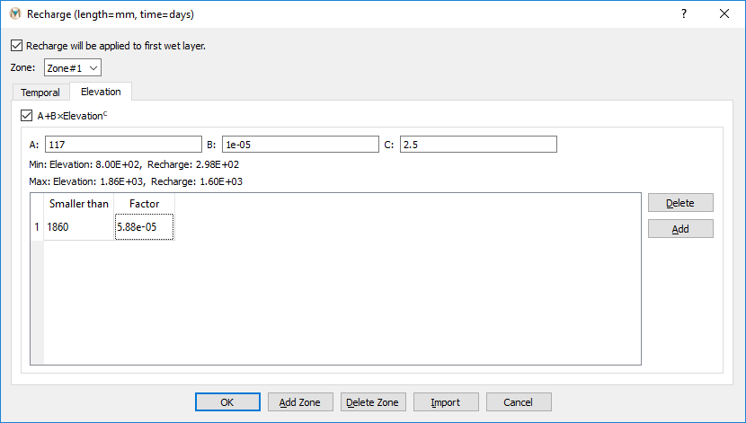
Figure 1.51 Parameters for orographically controlled recharge

To assign recharge zones to the model domain, select the “List” tab in the “Control Panel” pane. Expand the “Element” item and double-click “2D Plane” (Figure 1.52).

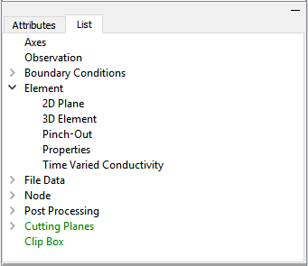
Figure 1.52 The location of the “2D Plane” plot item

While the 2-D plane is selected in the “Control Panel” pane, select the “Attributes” tab and select “Recharge” from the “Color By” drop-down menu (Figure 1.53).

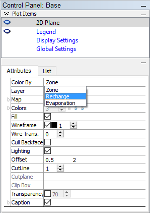
Figure 1.53 The “Attributes” of the “2D Plane” plot item

Click the “Select” tool and drag a box around the mountainous region of the model domain to assign Recharge Zone #1 to the model. After selecting the elements, press the [Enter] key, and the “Select Recharge Zone” dialog box appears (Figure 1.54). Make sure that Zone #1 is selected (Figure 1.54) and then click “OK.”

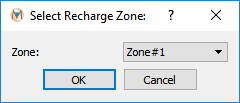
Figure 1.54 The “Select Recharge Zone” dialog box

Repeat the steps above, but this time select the elements that form the lowland area of the model domain and select “Zone#2” from the “Select Recharge Zone” dialog box. When assignment of the recharge zones is complete, the result should appear similar to what is shown in Figure 1.55.

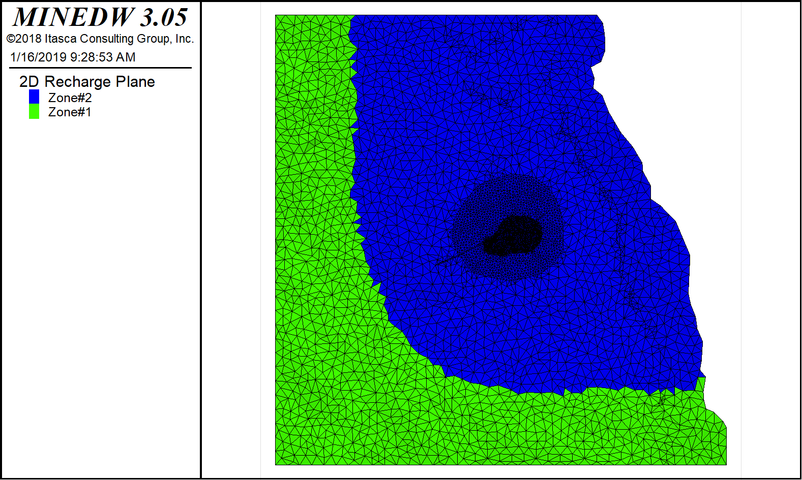
Figure 1.55 Assignment of recharge zones to the model

Step 12. Adding Evaporation

To finalize the boundary condition definitions, evaporation will need to be added to the model. Unlike recharge, only one evaporation zone can be created. Evaporation rates can vary over time or be constant for a transient simulation. For the steady-state simulation, a constant-rate evaporation zone will be used.

To create an evaporation zone, select “Evaporation” under the “BCs” menu. The “Define Evaporation Zones” dialog box appears. Enter the evaporation values in the appropriate dialog boxes (Figure 1.56). For this tutorial, evaporation will be simulated as constant over time. Once the appropriate evaporation values have been entered in the “Define Evaporation Zones” dialog box, click “OK” to finalize the evaporation zone definition.

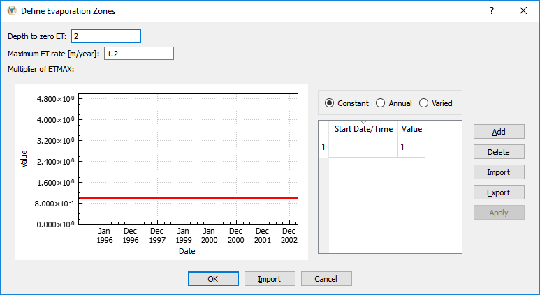
Figure 1.56 The “Define Evaporation Zones” dialog box

Now that the evaporation zone has been created, it needs to be assigned to the mesh. To assign evaporation to the mesh, add a “2D Plane” plot item and select “Evaporation” as the “Color By” attribute. Next, select all the elements that are not adjacent to the “River” or “Pond” boundary conditions. It may be easiest to use the “Select With Polygon” tool and select elements that do not border the “River” or “Constant Head” boundary conditions (Figure 1.57). When the appropriate elements have been selected, press [Enter] to open the “Select Evaporation Zone” dialog box. Select “Evaporation” in the drop-down box and then click “OK” to finalize the evaporation zone.

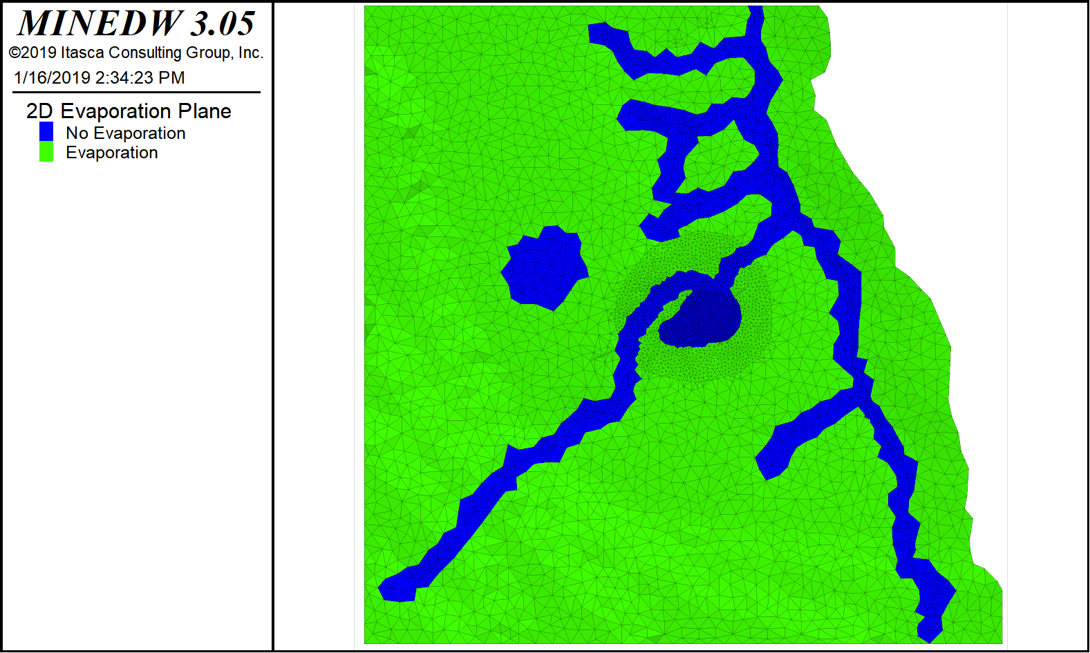
Figure 1.57 The assigned evaporation zones

Step 13. Saving the Project

After completing the model setup, click “File” on the Main Menu banner. Select “Save Project” to save the changes to the project.

1.4 Running the Model

To run the model, click “Run” on the Main Menu banner, then select “Validate.” The “Validate” function checks for errors, such as defining a constant-head level for a constant-head node that is lower than the node itself, and for multiple assignments to a node, such as assigning two constant-head boundary conditions to one node. The function also summarizes the model construction, such as the number of nodes, elements, pumps, etc. After reviewing the model, click “Validate,” and MINEDW will check for errors in the model. Any errors will be highlighted in the window. If errors are found, review the relevant definitions by following the steps outlined in the previous sections. If no errors are found, click “OK” to complete the validation process.

If the model passes the validation process, then click “Run” again and select “Create Data Set.” Select the folder where you want to create your input data set. All input files for MINEDW model runs will be created in the chosen directory. NOTE: FILES MUST BE CREATED BEFORE RUNNING THE MODEL. Next, click “Run” on the Main Menu banner and select “Execute” to run the model. A window will appear showing the simulation progress.

1.5 Results

MINEDW has several functions that allow the user to do most of the post-processing they will need.

Under the “Element” plot item category on the “List” tab, the “3D Element” plot item can be used with the “Isoline” or “Isosurface” plot items under “Node” to plot geology and head, pore-pressure, or water-table contours. The “2D Contour” and “3D Contour” plot items can also be used to plot contours or color floods of head, pore pressure, or the water table.

To visualize the simulation results, click “Results” on the Main Menu banner and then choose “Read Results.” Select the .PLB file from the folder where MINEDW was executed. (Note: The .PLB file is a binary file that contains the calculated head over time.) MINEDW will read the entire file.

Water-Table Contour:

To plot the water-table contours, select the “List” tab from the “Control Panel” pane, expand the “Node” item, and then double-click “2D Contour” (Figure 1.58).

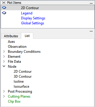
Figure 1.58 The “2D Contour” plot item

On the “Attributes” tab, from the “Color By” drop-down menu, select “Water Table.” The water-table contour appears in the View Pane. To view the desired time step, enter it in the variable field or move the time step slider bar found on the Main Menu banner. The slider is shown in Figure 1.59. For the steady-state simulation, view the last time step (time step 100 in this tutorial).

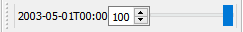
Figure 1.59 Time step slider

To export the water-table contour as a bitmap, select “Export Base” from the “File” item on the Main Menu banner and choose “Bitmap.” The exported bitmap is provided in Figure 1.60.

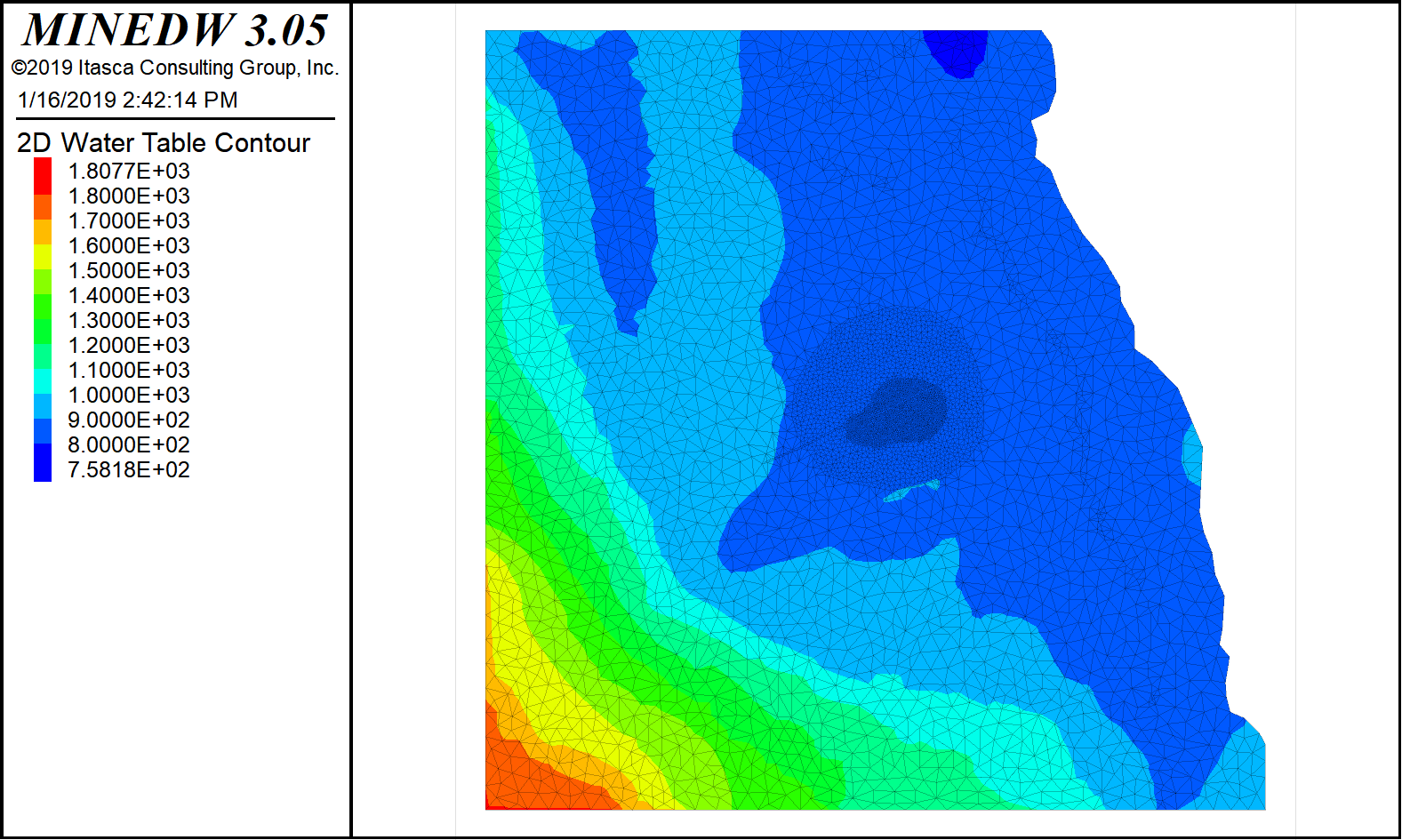
Figure 1.60 Water-table contours from steady-state simulations

2-D or 3-D Head Contour:

To create a 2-D or 3-D contour plot of the head distribution, select the “Node” item under “List” on the “Control Panel” pane and double-click on either “2D Contour” or “3D Contour.” A 2-D contour is ideal for creating a 2-D color flood image of head distribution within any of the model layers, while a 3-D contour item is best for creating 3-D images of head distributions or cross sections. Figure 1.61 is a cross section through the model displaying head. To recreate this image, choose “3D Contour” and then choose “Head” in the “Color By” drop-down menu on the “Attributes” tab. Next, double-click on “Plane” located under “Cutting Planes.” Enter the following values for the “Plane” on the “Attribute” tab: Origin = (466236, 9.07489e+6, 250), Normal = (-0.429008, 0.903301, 0) Dip/DD = (90, -25.4046). Then click the “Snap View” button. Note: Cross sections can be created using the “Create Plane with two selected points on the plot” tool, but the location of the cross section is not as precise. Select the “3D Contour” in the “Plot Items” pane and then expand the “Cutplane” item on the “Attributes” tab. The cross section can easily be modified to display pore “Pressures” or “Head Difference” by selecting the appropriate item from the drop-down menu next to “Color By” on the “Attributes” tab for the “3D Contour” plot item.

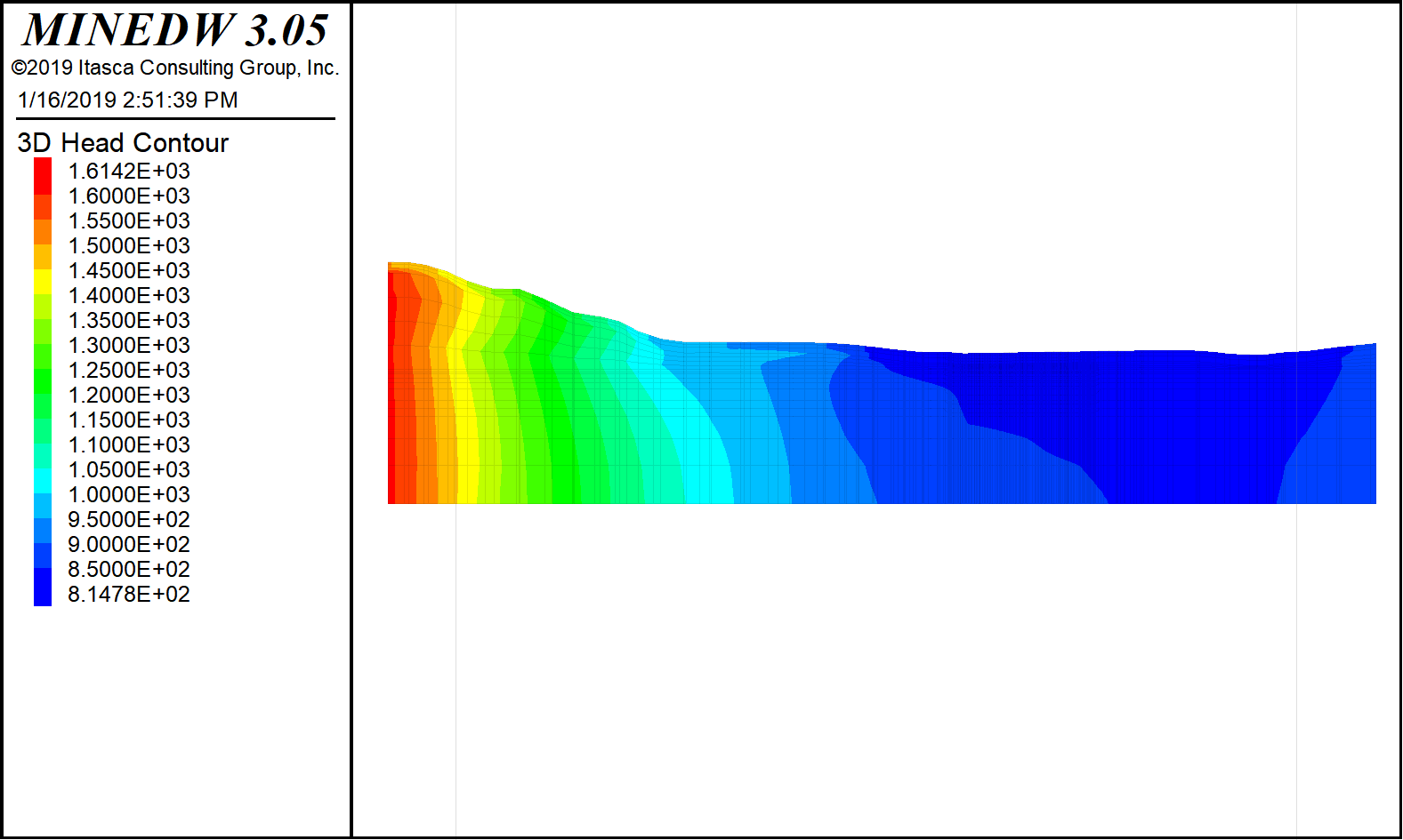
Figure 1.61 A 3-D cross section of head exported from MINEDW

Geologic Cross Section and Water Table:

MINEDW can create cross sections showing the geology represented in the model overlaid by the groundwater table. To construct a figure similar to the one shown in Figure 1.62, select “3D Element” (found under “Element”) from the “List” tab in the “Control Panel” pane. Next, add a “2D Contour” (under “Node”) and select “Water Table” from the “Color By” drop-down menu on the “Attributes” tab. Finally, create a cross section using the “Create Plane with two selected points on the plot” tool. Colors for both the “3D Element” and “2D Contour” plot items can be modified by expanding the “Contour” attribute and choosing a different color ramp.

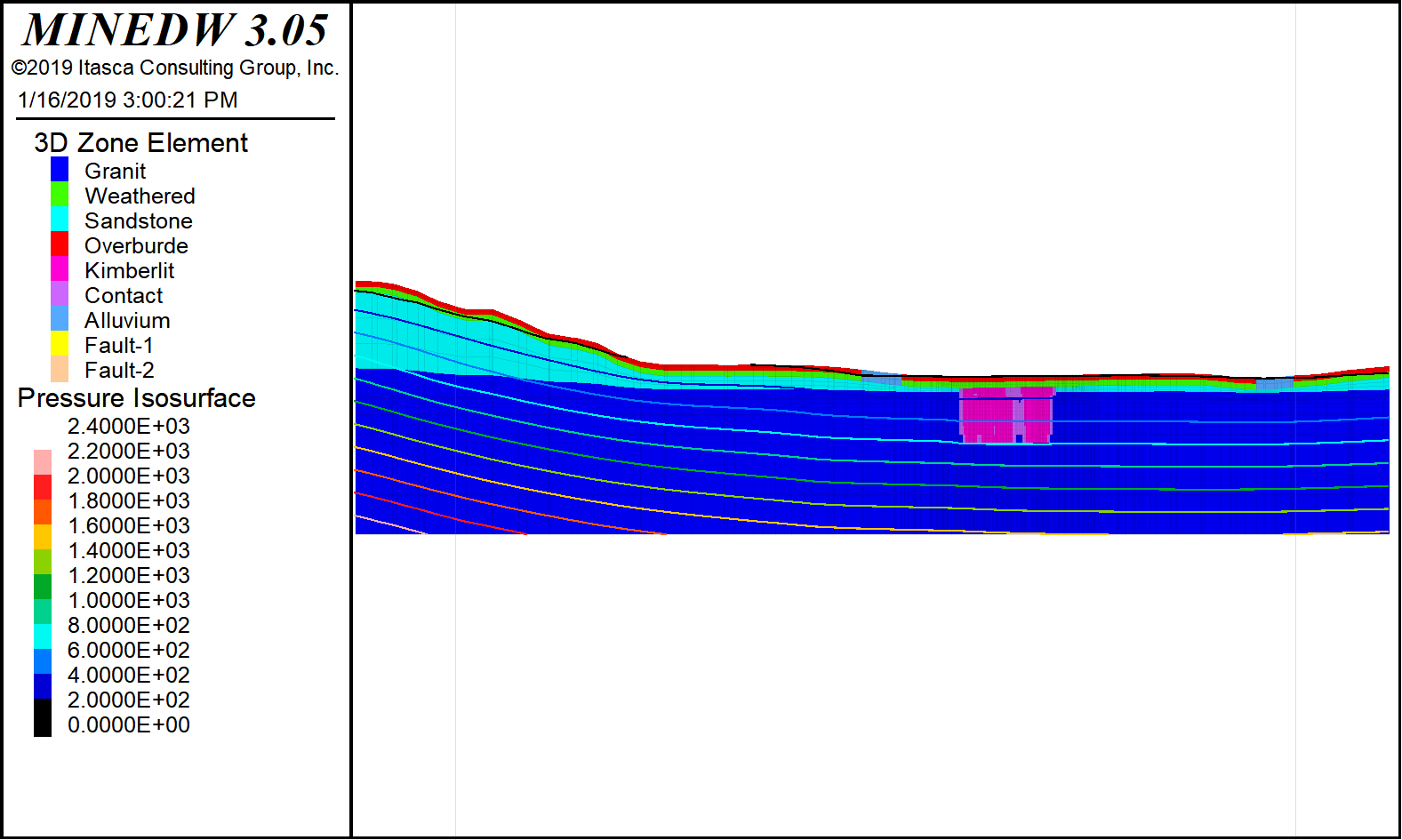
Figure 1.62 A cross section of the geology and water table