Tutorial 2 - Open Pit Mining

2.1 Problem Description

Tutorial 2 demonstrates the setup of a transient-state simulation including an open pit, a ZOR, pumping wells, and a pit lake.

Tutorial 2 uses the same model as Tutorial 1. The simulation results from the steady-state simulation (Tutorial 1) are used as the initial conditions for Tutorial 2. In this part of the document, the procedure for creating a mining plan, ZOR, pit lake, and variable-flux boundaries will be discussed step by step.

Step 1. Opening the Project File

The model created in Tutorial 1 is used for this problem. To open the project file created in the first tutorial, click “File” on the Main Menu banner, then select “Open Project.” The “Load a MINEDW Project File” dialog box appears, as shown in Figure 2.1.

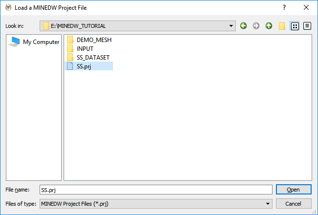
Figure 2.1 The “Load a MINEDW Project File” dialog box

Select the project (.PRJ) file and click “Open.” Click “File” on the Main Menu banner, then select “Save Project As” to save the project as a different .PRJ file for the transient simulation.

Step 2. Defining Project Properties

To define a project property, click “Project” and then select “Project Property.” The “Project Properties” dialog box shown in Figure 2.2 appears. Make sure that all the fields shown in Figure 2.2 contain the values shown in Figure 2.2. For transient simulations, select the “Transient” option and then click “OK.”

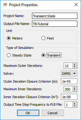
Figure 2.2 The “Project Properties” dialog box

Step 3. Defining Model Time Steps

To define the time steps for the project, click “Project” on the Main Menu banner, then select “Time Steps.” The “Set Up Time Step” dialog box (Figure 2.3) appears. Set the “Maximum Time Steps” to 300. The first time step is 1 January 1995. The time-step length will be one month. For transient simulations, the multiplication factor (as discussed in Tutorial 1) is 1 and the time-step length is defined in the “Set Up Time Step” dialog box. Ensure that the “# of time steps for this simulation” slider is set to 300 and that the “Start at Time Step” combo box is set to 1 and click “OK.”

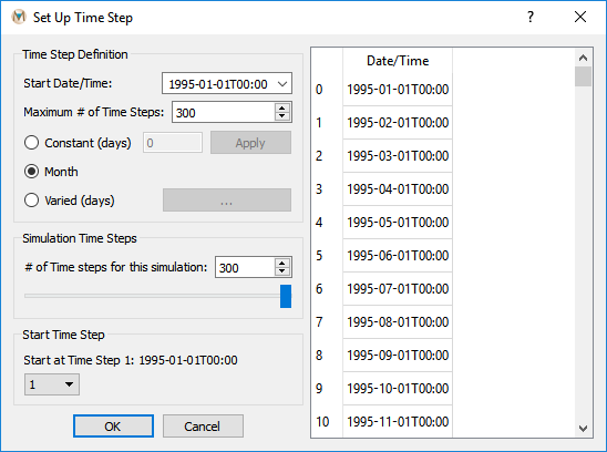
Figure 2.3 The “Set Up Time Step” dialog box

Step 3. Defining Initial Heads

To define initial heads, click “Project” on the Main Menu banner, then select “Initial Heads.” The “Set Up Initial Head” dialog box appears. Choose the “Varied” option and select the water levels file (“*.MDL”) created during Tutorial 1 by clicking on the “…” button as shown in Figure 2.4, then click “OK.”

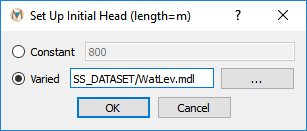
Figure 2.4 The “Set Up Initial Head” dialog box

Step 4. Creating a Mining Plan for an Open Pit

The easiest method to create a mine plan in MINEDW is to obtain .DXF files of the pit topography at various points in time (e.g., at the end of every year of mining). Each .DXF file will need to be converted to a data file containing X, Y, Z coordinates of the pit surface for interpolation of the mine plan to a mining input file for MINEDW. In this example, there are 11 years of mining. .DXF files of the planned pit shape at the end of each year of mining are found in the “INPUT/OPENPIT” file directory.

On the “List” tab, double-click on “File data,” then double-click on “DXF.” The “Attributes” tab will appear. To select the .DXF file for Year 1, select the “+” next to “File” as shown in the red box in Figure 2.5, browse to the file, select it, and click “Open.” Next. select the icon next to “To Data File” at the bottom of the “Attributes” tab to save the information from the .DXF file as a data (“*.DAT”) file. Be sure to use the same file name as the .DXF file to name the “*.DAT” file; otherwise, the next step will not work. Repeat these steps for the next 10 years of mining.

For any mining plan that is created in MINEDW, a pit footprint is required (e.g., the ultimate pit boundary) to define the nodes that will be used for interpolation. This boundary needs to be defined in a .BLN file format (Appendix B). This boundary is always the first record in any mining schedule when creating an open-pit mining plan. This file defines the perimeter of the open pit and does not contain ground-surface elevation information because all ground-surface elevations are assumed to be the top of the mesh.

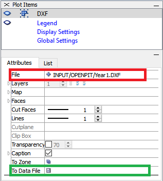
Figure 2.5 Reading a .DXF file and saving as a data file

To create the mining plan, on the Main Menu banner, click “Mining,” then select “Create Mining Plan.” The “Create Mining Plan” dialog box (Figure 2.6) appears. The date, file name, and interpolation method can be entered manually by typing in the information under “Date,” “File/Elevation,” and “Interpolated With,” respectively. Another option is to select an input file known as a Mining Schedule file (Appendix B) containing this information. Itasca has created a Mining Schedule file to illustrate this process. To use it, select the “Open” button and select the file “INPUT/OPENPIT/MINE_SCHEDULE.DAT.” This file contains the dates and file names, as shown in Figure 2.6. After importing the mine plan file information, enter a file name for the new mining plan file in the “Created Mining Plan File Name:” box (for example, “MINE_FILE.DAT”) at the bottom of the “Create Mining Plan” dialog box (Figure 2.6). In order to create a mining file, all input mining files must be located in the same directory (in this example, the files “MINE_SCHEDULE.DAT,” “ULTIMATE.BLN,” “YEAR1.DAT,” “YEAR2.DAT,” etc. were moved from “INPUT/OPENPIT” to the main simulation directory). Next, click the “Options…” button to open the “Mining Plan Interpolation” dialog box. Uncheck the box next to “Not interpolated if no data found in Range.” This will exclude locations that do not have associated elevation data. Click “OK” on the “Mining Plan Interpolation” dialog box to accept the changes and then click “OK” on the “Create Mining Plan” dialog box to create the mining plan file for the MINEDW model.

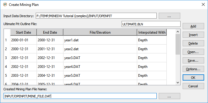
Figure 2.6 The “Create Mining Plan” dialog box

To assign a mining file to the model, click “Mining” on the Main Menu banner and select “Open Pit.” The “Open Pit” dialog box appears (Figure 2.7).

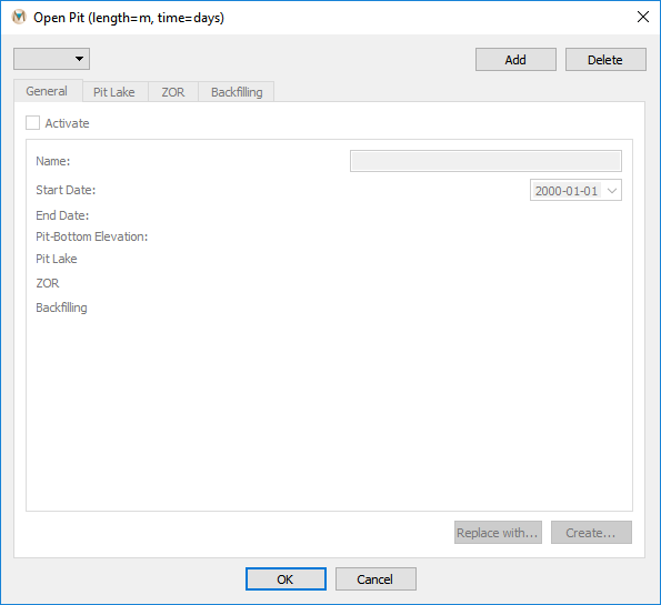
Figure 2.7 The “Open Pit” dialog box

Click “Add” and browse to the newly created mining file, select it, and click “Open.” After importing the mining file, the “General” tab in the “Open Pit” dialog box will show the “Start Date” and “End Date” for mining as well as the “Pit-Bottom Elevation.” This tab will also indicate whether a “Pit Lake,” “ZOR,” or “Backfilling” will be simulated. Immediately after importing the mining file, these options should indicate that none will be simulated. Steps 5 through 7 describe how to add these features to a model simulation after creating and importing a mine plan. No additional open-pit mines will be simulated in this tutorial, but if required, multiple open-pit mines can be added to the model for simulation by repeating the steps described above for creating and importing mining files.

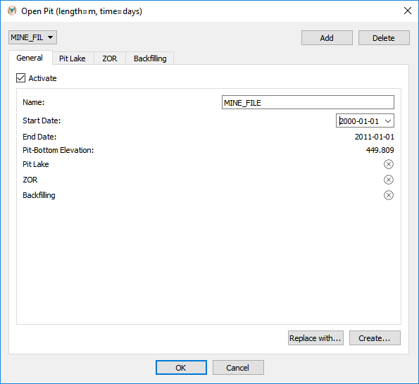
Figure 2.8 The “Open Pit” dialog box showing the “General” tab

Step 5. Creating a Zone of Relaxation for an Open Pit

In MINEDW, time-variant hydraulic conductivity (K) can be simulated for situations such as a ZOR around open-pit excavations, backfilling operations, longwall and room-and-pillar coal mining, and freeze-thaw conditions.

To create a ZOR for this open-pit simulation, select “Open Pit…” from the “Mining” drop-down menu on the Main Menu banner. The “Open Pit” dialog box (Figure 2.8) appears. Select the “ZOR” tab to create the ZOR. MINEDW offers two options for defining the thickness of the ZOR: (1) As a ratio of the pit depth or (2) by a user-defined thickness (both options are discussed in detail in Section 7.6.4 of the MINEDW manual). In this tutorial, the ZOR will be defined as a ratio of the pit depth and divided into two layers. To create the ZOR, check the box next to “ZOR thickness = 1/” and enter “3” as the denominator in the box. In the box next to “# of Additional ZOR Layers,” ensure that the value is “1.” MINEDW will add a default layer to the one layer defined by the user for a total of two layers within the ZOR. Only the thickness of the first ZOR layer needs to be defined because the remainder of the ZOR will automatically be assigned to the default ZOR layer created by MINEDW. The thickness of each layer is defined as a percentage of the total ZOR thickness. In this tutorial, both ZOR layers will be equal in thickness (i.e., each layer will be 50% of the ZOR) (see Figure 2.10).

Figure 2.9 The “Open Pit” dialog box showing the “ZOR” tab

Next, click “Search ZOR Units,” located at the bottom of the dialog box. The geological zones that lie within the defined ZOR will appear (Figure 2.9). The numbers next to each geological unit represent the factor by which the K in each ZOR layer will change. The default is 1, or no change in K values. Numbers greater than 1 represent an increase in the K values (i.e., to double the K values, enter “2”), while numbers less than 1 represent a decrease in the K values.

In this tutorial, the K values are 10 and 2 times greater than the original K values. In the “ZOR Definition” dialog box, enter “10” next to the units in “Layer#1” except for the “Overburden” and “Alluvium” zones, as they will be removed prior to mining (leave as 1). See Figure 2.10 for more details about assigning values to the second layer of the ZOR. After entering the appropriate data in the “ZOR” tab of the “Open Pit” dialog box, click “Create” and then check the box next to “Activate” (this option only becomes active after the ZOR has been correctly defined). Finally, click “OK” at the bottom of the dialog box to apply the changes to the model and exit the “Open Pit” dialog box.

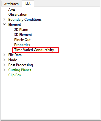
Figure 2.10 The “Time Varied Conductivity” plot item

Once a ZOR has been created, it can be visualized by selecting the “List” tab in the “Control Panel” pane and then selecting the “Time Varied Conductivity” plot item under the “Element” group (Figure 2.10). The ZOR that was created is shown in Figure 2.11.

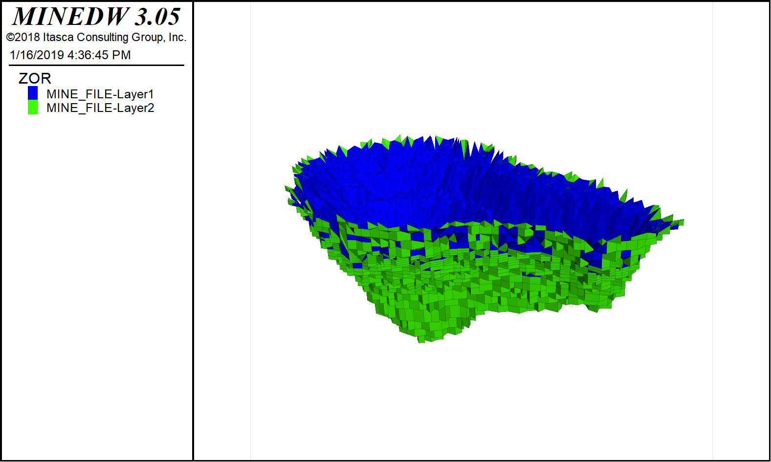
Figure 2.11 ZOR defined in the model

Step 6. Open-Pit Backfilling

Backfilling may be used in some mining applications to prevent the formation of a pit lake or to dispose of tailings after mining has ceased. To add backfilling, select the “Backfilling” tab (Figure 2.12). Check the “Activate” box and define the “Implement Date” for backfilling. The “Implement Date” of backfilling must be before the “Start Date” of pit-lake formation. MINEDW does not support the backfilling of an existing pit lake and will automatically adjust the “Start Date” or “Implement Date” for pit-lake formation or backfilling operations to prevent this. Backfilling operations are simulated in one time step rather than progressive backfilling over multiple time steps. The backfill elevation can be defined as constant by checking the “Constant Elevation” option and entering a value. Otherwise, if more detailed information is available for the backfill, “Varied” can be selected. For this tutorial, check the “Constant Elevation” radio button and enter the elevation of the final backfill (Figure 2.12). Finally, the hydraulic parameters for the backfill can be selected from the drop-down list labeled “Backfill Unit” (Figure 2.12). The entire backfilled zone will have the same hydraulic properties and cannot be subdivided. When the “Backfilling” parameters are completely defined, click “OK” in the “Open Pit” dialog box to ensure the changes that were made are saved.

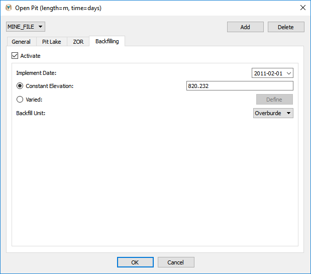
Figure 2.12 The “Backfilling” tab

Step 7. Creating a Pit Lake

When mine operations and dewatering activities cease, a pit lake may form if the pit-bottom elevation is below the recovering water-table elevation. To simulate the pit-lake formation in MINEDW, select “Open Pit” from the “Mining” drop-down menu. In the “Open Pit” dialog box, ensure the “MINE_FILE” plan is showing in the drop-down box in the upper left-hand corner and then select the “Pit Lake” tab (Figure 2.8). Enter a date in the “Start Date:” box for the start of the pit-lake formation. Next, enter a value for “Initial Lake Elevation.” This value must be equal to or greater than the ultimate pit-bottom elevation. In this tutorial, the open-pit “Initial Lake Elevation” should be the minimum pit-bottom elevation of 450 m (the bottom of the pit at the end of mining, Figure 2.8). If evaporation from the pit-lake surface is to be considered, enter the evaporation rate value in the “Evaporation (mm/yr)” box. For this model simulation, evaporation is assigned a rate of 1,200 millimeters per year (mm/yr). Enter the number of stages to use to calculate the pit-lake volume in the “# of Stages” box. For this example, 15 stages (Figure 2.13) are used. Increasing the number of stages will give a more accurate estimation of inflow to the open pit but may cause convergence problems in the model simulation. As a rule of thumb, start with stages that are approximately 50 m in depth; if greater accuracy is required, increase the number of stages. Next, check the box next to “Activate” and click “OK” at the bottom of the dialog box to apply the changes to the model and exit the “Open Pit” dialog box.

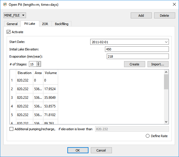
Figure 2.13 The “Pit Lake” tab

Step 8. Adding Pumping Wells

Pumping wells are extensively used in open-pit dewatering systems. In MINEDW, there are three options available for pumping wells, all of which are explained in detail in the MINEDW Manual section 7.4.4. Pumping wells can be defined in the model by defining pumping rates, specified heads, or pumping rates with a lowest pumping elevation (LPE).

“Pumping Rate,” “Pumping with LPE,” and “Specified Head” wells will be added in one step. During the calibration and predictive simulations, it is important to use the correct type of pumping well. “Pumping Rate” and “Pumping with LPE” are two good choices for wells to use during calibration because the user can assign actual pumping rates from the field to these wells in the model. A “Specified Head” well is useful for predictive simulations, as it allows the user to specify the level to which they wish to lower the phreatic surface without needing to manually adjust the pumping rate.

To add pumping wells to the model, from the “Control Panel” pane, select the “List” tab, expand the “Node” item, and then double-click “3D Contour.” Next, toggle to layer 27 using the toggle buttons next to the “Layer” attribute on the “Attributes” tab (Figure 2.14). The layer where the pump is to be simulated must be selected in order for the user to correctly construct the pumping wells in the model. Nodes above the pumping wells are then used to simulate the well screen.

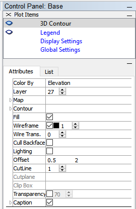
Figure 2.14 The “Control Panel” pane with the “Attributes” tab selected to show the correct layer for pumping wells

In the MINEDW main window, click the “Select” button on the Main Menu banner. To locate the pumps in the model domain, use the pump locations that were used to create the mesh. Add a “Point Data File” plot item, which is found under the “File Data” item in the “Control Panel” to the View Pane (Figure 2.15). Use the “File” attribute on the “Attributes” tab to open the “Select Data File” dialog box. Use the “Select Data File” dialog box to navigate to the location where the input data for these tutorials are located and select the “Pumps.Dat” file in the “INPUT/MESH_INPUT/DAT” directory.

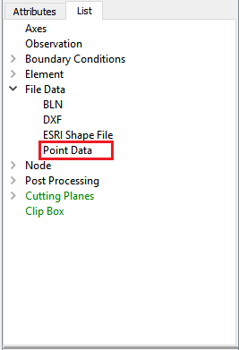
Figure 2.15 The “Point Data” plot item

Select the nodes below the points now displayed in the View Pane and then press [Enter]. In the “Assign Properties for Nodes” dialog box, select the “Add to Pumping Wells” option (Figure 2.16), then click “OK.” For this tutorial, the goal will be to dewater the open pit during active mining using any combination of the three pumping well types.

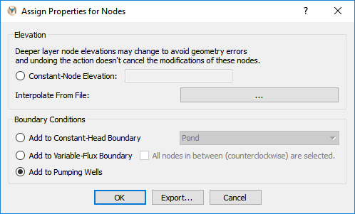
Figure 2.16 The “Assign Properties for Nodes” dialog box showing the “Add to Pumping Wells” option selected

Next, open the “Pumping Well” dialog box by clicking on “BCs” on the Main Menu banner, then select “Pumping Well.” The newly added pumping well nodes appear in the “Pumping Well” dialog box (Figure 2.17).

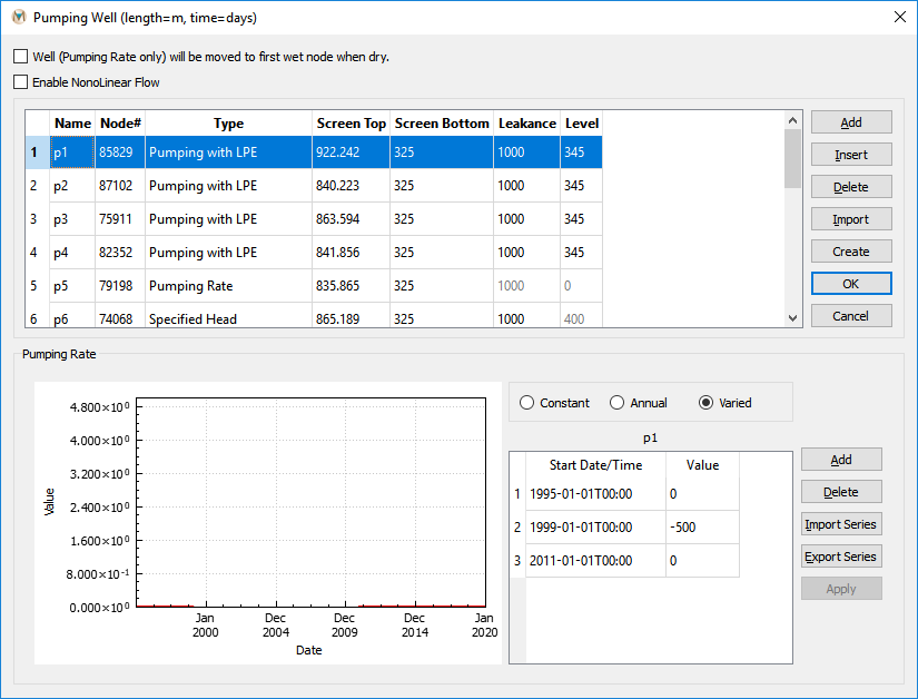
Figure 2.17 The “Edit Pumping Wells” dialog box

Set the “Type” as “Pumping with LPE” for the first several pumping wells (Figure 2.16 and Figure 2.17). Define the “Screen Top” (initial screen top will be the ground-surface elevation), “Screen Bottom” (initial screen bottom will be the selected node elevation), LPE (“Level”), and pumping rate for all LPE wells. Choose a starting time for pumping to begin; this may be one of the parameters used to achieve dewatered conditions through the life of the mine. To turn pumping off, set the pumping rate to -9,999,999 in the last pumping-rate record of the dialog box. It is important that the last pumping-rate record be a large negative number if pumping is to be turned off. If it is not the last record or it is not a large negative number, MINEDW will not recognize that the well is to be turned off and will continue to extract water at that well. Pumping in this tutorial should end on or before the end of mining (Figure 2.17). If the pumping rate changes with time, go to the lower right window shown in Figure 2.17 to include pumping rates for different times. Pumping-rate data can be imported directly using the “Import” function at the lower right of the dialog box. The structure of the pumping rate file is described in Appendix B.

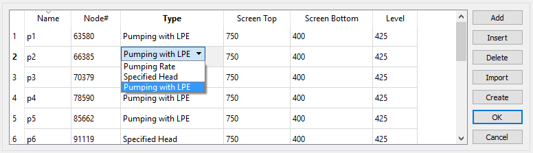
Figure 2.18 The “Edit Pumping Wells” dialog box showing the pumping well types available in MINEDW

For “Pumping Rate” wells, select “Pumping Rate” under “Type” (Figure 2.18) and then enter the “Screen Top” and “Screen Bottom” information. In the time-series window, choose whether the pumping rate is “Varied,” “Annual,” or “Constant” and then enter the pumping-rate data. Pumping for the tutorial model should end at the end of mining or before, so ensure that the pumping rate is 0 on or before 1 January 2011.

“Specified Head” wells can be used to lower the head in the groundwater system surrounding the well to a specified head level. This feature is useful for predictive simulations in which the pump and well must be designed to meet the dewatering objectives but the pumping rate required to achieve the objective is unknown. To add “Specified Head” wells to the model, select “Specified Head” under “Type” and then enter the information for “Screen Top” and “Screen Bottom” and enter the specified head values in the rate time-series window below. For this tutorial, the “Specified Head” wells will be deactivated on 1 January 2011 by entering “-9,999,999” in the pumping-rate window located in the lower right of the “Pumping Well” dialog box. Any pumping-rate information entered in the pumping-rate window is ignored for “Specified Head” wells because abstraction rates are estimated by the hydraulic properties of the aquifer and hydraulic head at that point. The only value entered in the pumping-rate box that is recognized by MINEDW for “Specified Head” wells is a large negative number, such as “-9,999,999,” which will deactivate the “Specified Head” well.

Step 9. Defining the Boundary Conditions

Variable-Flux Boundary

A “Variable-Flux” boundary condition is assigned from the top of the model to the bottom along portions of the model domain. Ensure that Layer 5 is selected by clicking on the “Attributes” tab in the “Control Panel” pane and checking that “Layer” is set to 5, as shown in Figure 2.19.

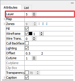
Figure 2.19 The “Attributes” tab

From the MINEDW main menu, click the “Select” button on the Main Menu banner.

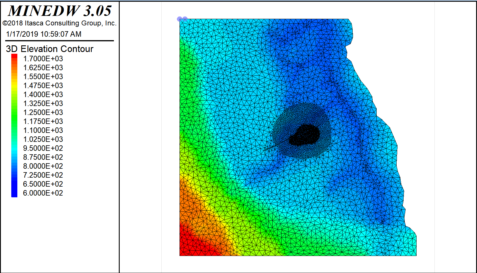
Figure 2.20 The View Pane showing the first and last node of the variable-flux boundary

Select the beginning node (node at top left corner) and ending node (the next node to the right) (Figure 2.20). The order of selection of the nodes is important because MINEDW will assign the nodes between the two selected nodes to the variable-flux boundary condition in a counterclockwise direction. After selecting the two nodes, press [Enter]. The “Assign Properties for Nodes” dialog box appears (Figure 2.21). Select “Add to Variable-Flux Boundary” and check the “All nodes in between (counterclockwise)” box, as shown in Figure 2.21 below. Enter “32” or whatever layer is the bottom layer in the “From Current Layer #1 To” box on the right.

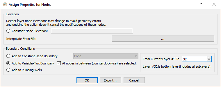
Figure 2.21 The “Assign Properties for Nodes” dialog box showing the “Add to Variable-Flux Boundary” option selected

All nodes between the selected beginning node and ending node will be selected and assigned as a variable-flux boundary condition. The assignment will be for multiple layers since “32” was entered as the bottom layer, as shown in the dialog box above. Click “OK.”

The flow rates from the constant-head boundary condition around the perimeter of the model should be imported as flow rates for the variable-flux boundary condition that was just added to the model. To do this, click on “BCs,” then select “Variable Flux” to open the “Variable-Flux Boundary” dialog box. At the bottom of the “Variable-Flux Boundary” dialog box is the “Import From DRN File” button. Click on this button to open the “Open Variable Flux File” window. Use this window to browse to the location where the steady-state simulation was conducted and select the file with the .DRN extension and click “Open.” Flow rates for the variable-flux boundary condition will be imported. Check the box next to “Apply Constant Flux From Steady State Simulation” to apply the flow to the model simulation. Figure 2.22 shows the “Variable-Flux Boundary” dialog box with the imported flow rates at the bottom of the dialog box.

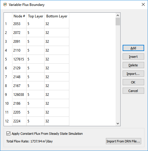
Figure 2.22 Imported flow rates

The next step will be to remove the constant-head boundary conditions around the perimeter of the model domain that were used in the steady-state simulation. The model should not have two types of boundary conditions assigned to one node. To remove the perimeter constant-head boundary condition, select the “Constant Head” item from the “BCs” menu on the Main Menu banner. Using the “Constant-Head Boundary” dialog box, select the “MtBlock” group from the “Group Definition” drop-down box. Next, click the “Delete” button located at the top center of the “Constant-Head Boundary” dialog box. A warning will appear indicating that the group is not empty and will ask if the user wishes to proceed. Click “Yes,” and this will delete this constant-head group. Repeat these steps for the “LowLand” group, but do not delete the “Pond” group.

2.2 Running the Model

To run the model, click “Run” on the Main Menu banner, then select “Validate.” If the model passes the validation process, click “Run” on the Main Menu banner and select “Create Data Set.” Select the folder where you want to create the data set. A data set must be created in order to run the model in MINEDW. Next, click “Run” on the Main Menu banner and select “Execute” to run the model. The following dialog box appears (Figure 2.23).

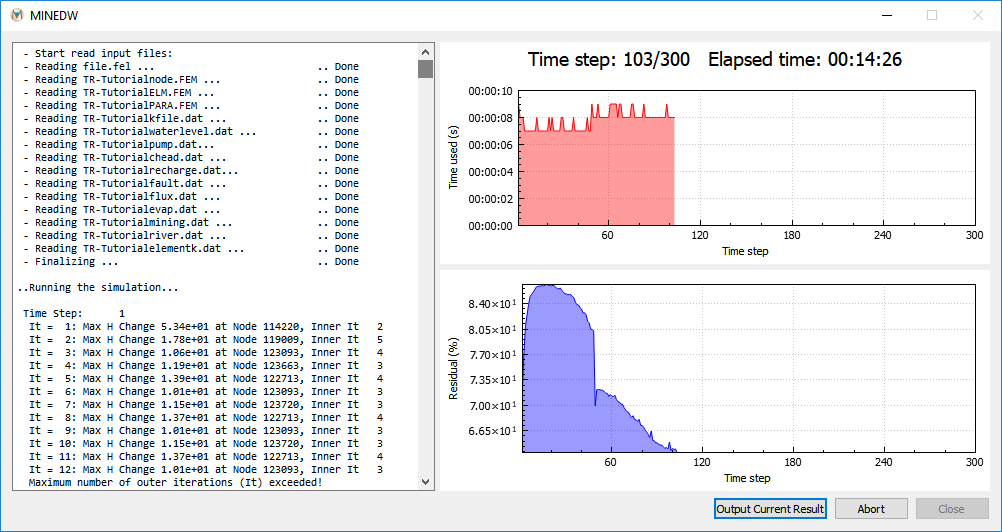
Figure 2.23 Screen display of output from the model run

2.3 Results

To visualize and export the simulation results once the model run has finished, click “Results” on the Main Menu banner, and then choose “Read Results.” Select the “*.PLB” file from the folder where MINEDW was executed. To view the desired time step, enter it in the variable field or move the time-step slider (found on the right side of the Main Menu banner, as shown in Figure 2.24) to the desired time step.

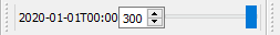
Figure 2.24 Time-step slider

Creating Monitoring Points

Model-calculated head values can be extracted using observations from either monitoring boreholes or piezometers. Monitoring boreholes will provide the head along a screened interval, while piezometers provide the head at a single vertical point. Observation locations can be defined by using the “Observations” function under “Results.” When “Observations” is selected from the “Results” drop-down menu, the “Edit Observations” dialog box appears (Figure 2.25). Select the “Monitoring Borehole” tab, click “Add” and enter the “Name,” “X” coordinate, “Y” coordinate, “Screen Top,” and “Screen Bottom” information for each observation point as shown in the figure below, and then click “OK.” To add “Piezometer” observation points, click on the “Piezometer” tab, then click “Add” at the top of the dialog box (Figure 2.26). This will add a piezometer location, but observation points, or “Transducers” as they are labeled in the legend, must be specified too. Each piezometer may have multiple transducers, each with its own X, Y, and Z coordinates. After adding a piezometer, click “Add” in the middle of the dialog box (Figure 2.26) to add a transducer. Define the X, Y, and Z coordinates of the transducer, then click “OK.” It is also possible to import the observation points from a text file that is space delimited. The observation file format is provided in Appendix B of the MINEDW manual. The easiest way to learn the file format that MINEDW requires is to first create one by defining a “Monitoring Borehole” and “Piezometer” and then exporting to a “*.DAT” file. This can be done by clicking the “Export” button at the bottom of the “Edit Observations” dialog box.

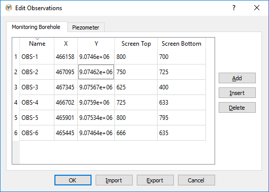
Figure 2.25 The “Edit Observations” dialog box

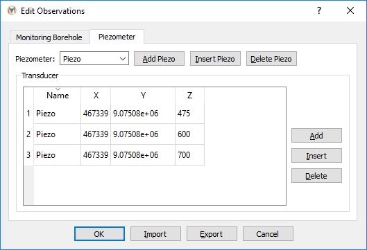
Figure 2.26 The “Edit Observations” dialog box with the “Piezometer” tab selected

Creating Hydrographs

To create hydrographs from simulation data, select the “Hydrograph” option from the “Results” drop-down menu on the Main Menu banner. The water-level data for the observation will be exported to a “*.DAT” file. The exported file includes time steps, the corresponding date, well identification (ID), and corresponding water-level data for the entire model run. The .DAT file can be imported into Microsoft^® Excel or other software to create tables and graphs.

Pit-Node Elevation and Water Table

The pit-node elevation and the water-table elevation can be plotted against time. To create this plot, click “Results” on the Main Menu banner, and then choose “Pit Node Elevation and Water Table.” The “Elevation of Pit Node” dialog box appears (Figure 2.27). Enter the “Node Number” on the left side of the window and then click “View.” For the specified node, the change in the water table beneath the selected pit node and the pit elevation will be plotted as shown in Figure 2.27.

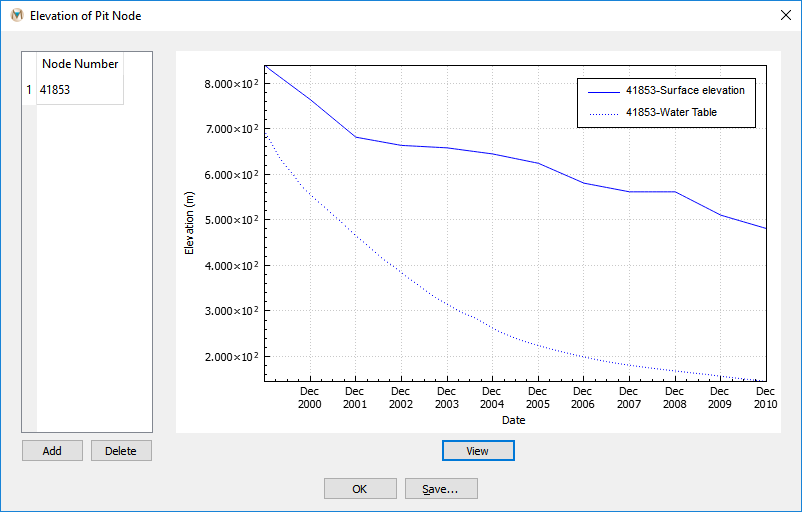
Figure 2.27 “Elevation of Pit Node” dialog box

If multiple nodes need to be plotted, click “Add” and insert the additional “Node Numbers.” Then click “View” again (Figure 2.28). The data used to create the pit-node and water-table plots can also be exported to a “*.DAT” file by clicking “Save.” In the “Save Pit Node Elevation File” dialog box, navigate to the location where the file is to be saved and enter a “File name,” then click “Save.”

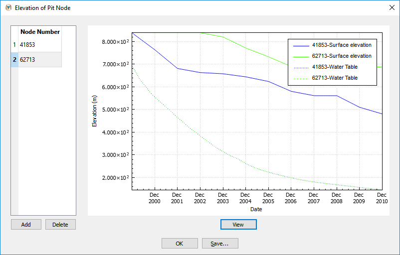
Figure 2.28 “Elevation of Pit Node” dialog box

Head Distribution in 3-D

To plot the head distribution, select the “List” tab from the “Control Panel” pane, expand the “Node” item, and then double-click “3D Contour” (Figure 2.29). Next, select the “Attributes” tab from the “Control Panel” pane and select “Head” from the “Color By” drop-down menu. The head distribution appears in the View Pane. By changing the time step with the time-step slider, the desired time step can be viewed.

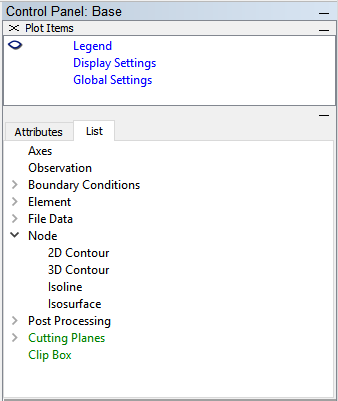
Figure 2.29 The “Control Panel” pane with the “Node” item expanded to show the “3D Contour” option

To export the head distribution in 3-D for the desired time step as a bitmap, select “Export Base” from the “File” menu on the Main Menu banner and choose the “Bitmap” option. The exported bitmap is provided in Figure 2.30.

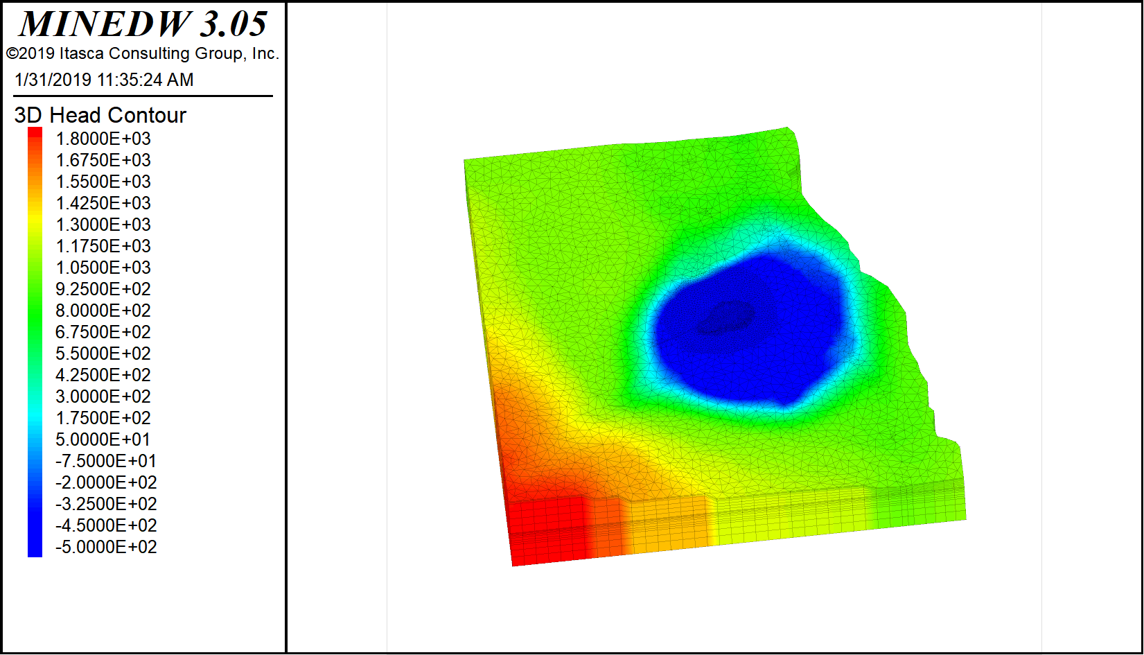
Figure 2.30 Screen display of head distribution in 3-D

Head Distribution Cross Section

With the “3D Contour” plot item still displaying in the View Pane, click the “Create Plane” tool on the Main Menu banner. Choose two points on the “3D Contour” plot item, and a cross section through the model domain will be created. Cycle through the time steps representing the model simulation by using the time-step slider or entering the desired time step in the time-step slider box. To visualize the cross section in 3-D, select “3D Contour” under the “Control Panel,” then expand “Cutplane” on the “Attributes” tab, and select the “Front” box (Figure 2.31).

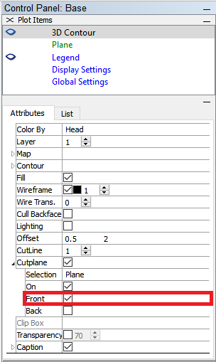
Figure 2.31 The “Control Panel/Plot Items” pane with the “3D Contour” item showing the “Attributes” tab

To export the head distribution in 2-D for the desired time step as a bitmap, select “Export Base” from the “File” item on the Main Menu banner and choose the “Bitmap” option. The exported bitmap is provided in Figure 2.32.

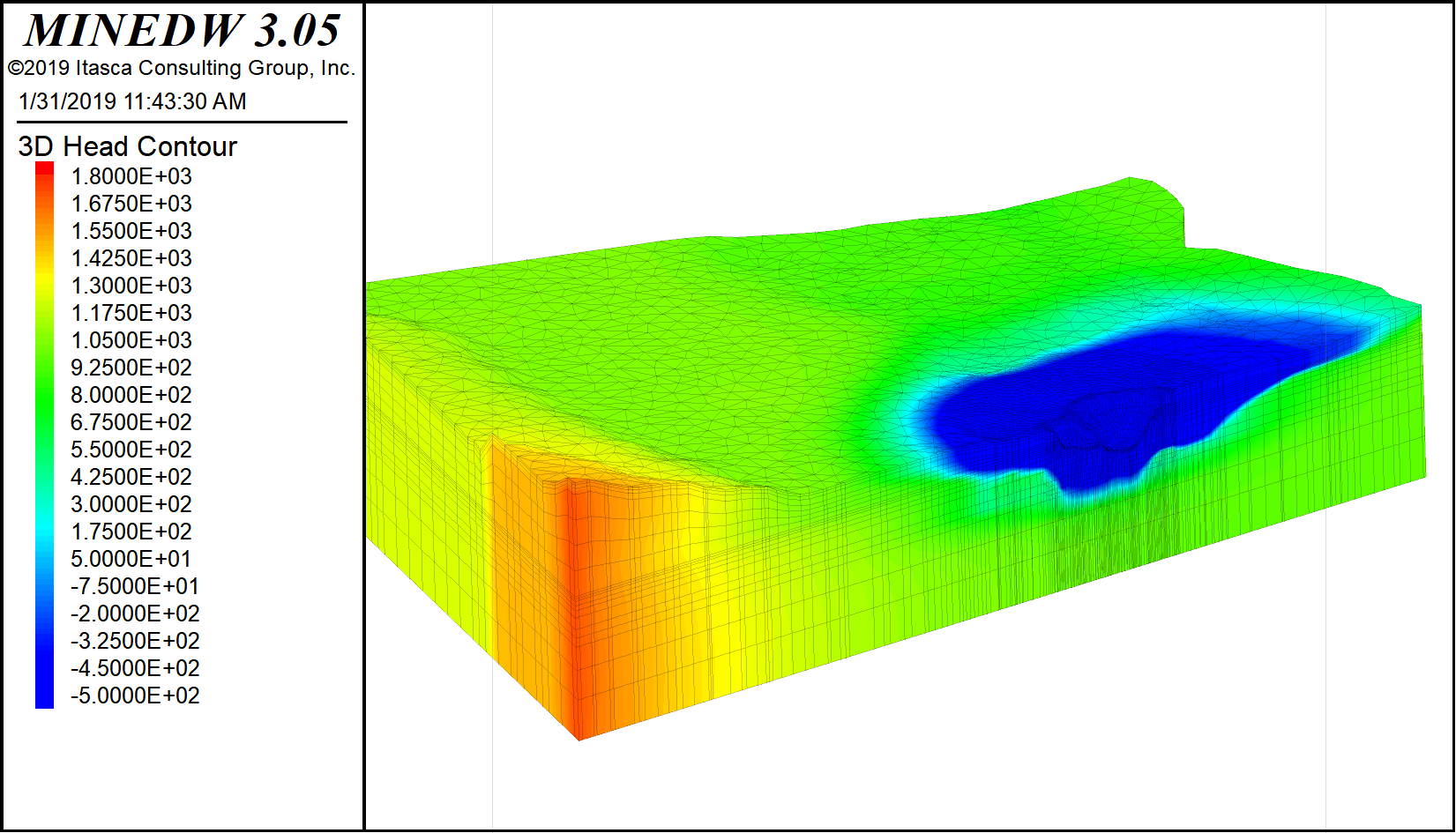
Figure 2.32 Screen display of output from the model run

Exporting Pore Pressures to a Different Grid in 2-D

MINEDW can export pore pressures in both 2-D and 3-D to a user-specified grid for use in other models, such as geomechanical models. The data are exported as a “*.DAT” file for use in geomechanical models. To export pore pressures in cross section (2-D), select the desired time step, then click “Results” on the Main Menu banner, and then choose “Export Cross-Section Pore Pressure.” The “Output Cross-Section Pore Pressure” dialog box appears (Figure 2.33).

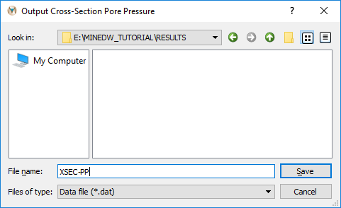
Figure 2.33 The “Output Cross-Section Pore Pressure” dialog box

Enter a file name and click “Save.” The “Grid – Export Cross Section Pore Pressure” dialog box appears. Choose the interpolation method (“Inverse Distance” or “Kriging”) and define the related parameters (Figure 2.34), then click “OK.” The pore-pressure data are saved to the specified file and can be imported into any contour-mapping software, such as Golden Software’s Surfer or ArcGIS ArcMap, to plot the contours.

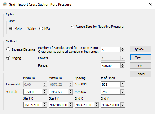
Figure 2.34 The “Grid – Export Cross Section Pore Pressure” dialog box

Exporting Pore Pressures to a Different Grid in 3-D

To export the pore pressures in 3-D, select the desired time step, then click “Results” on the Main Menu banner, and then select “Export Pore Pressure.” The “Output Pore Pressure” dialog box appears (Figure 2.35).

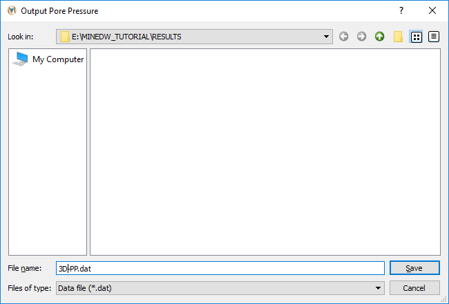
Figure 2.35 The “Output Pore Pressure” dialog box

Enter a file in the file name box at the bottom of the “Output Pore Pressure” dialog box and click “Save.” The “Grid – Export Pore Pressure” dialog box appears. Choose the interpolation method (“Inverse Distance” or “Kriging”) and define the related parameters (Figure 2.36), then click “OK.”

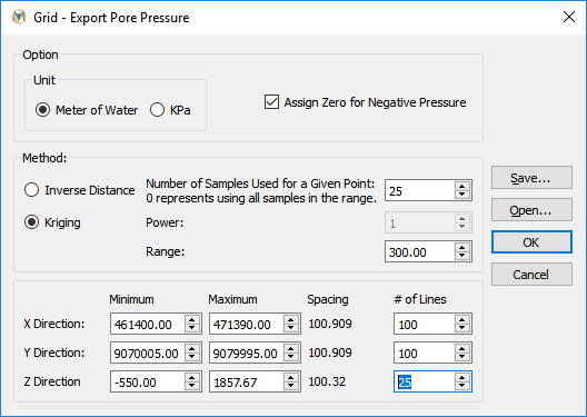
Figure 2.36 The “Grid – Export Pore Pressure” dialog box

The interpolated pore pressures are output as a “*.DAT” file and can be transformed and plotted using other commercial visualization software, such as EVS^© or Golden Software’s Voxler.

Seepage Component to Pit

MINEDW also computes the total seepage to a pit and contributions of each geological unit to seepage through time. To compute seepage to a pit, click “Results” on the Main Menu banner, and then choose “Seepage Component to Pit.” The “Flow of Pits” dialog box appears (Figure 2.37). Select the “*.SEP” file from the folder where MINEDW was executed. Select “Geological Units” to determine the contributions of each geological unit to seepage.

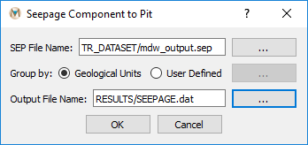
Figure 2.37 The “Seepage Component to Pit” dialog box

To define an output name and location, click on the “…” button to the right of the “Output File Name” box. The “Save Pit Flow File” dialog box appears (Figure 2.38). Type the name of the file to save at the bottom (e.g., “SEEPAGE”) and click “Save” and then click “OK.” The seepage file is created.

Figure 2.38 The “Save Pit Flow File” dialog box

The “SEEPAGE.DAT” file can be imported to Microsoft^® Excel or other plotting software to create time-series plots. Total seepage vs. time (Figure 2.39) and contributions from each geological unit to the seepage through time (Figure 2.40) can be plotted.

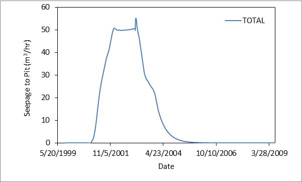
Figure 2.39 Total seepage to the pit through time

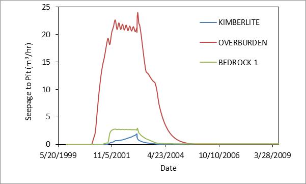
Figure 2.40 Contributions from each geological unit of seepage through time

Pit Lake – Water Level vs. Time

The water-level change in a pit lake can also be computed in MINEDW. To plot pit-lake level changes through time, import the “PITLEV.LAK” file from the folder where MINEDW was executed into Microsoft^® Excel. Figure 2.41 shows the pit-lake level changes through time. When analyzing the water levels in the pit lake, use only the water level after the pit lake begins to form and the water level begins to rise.

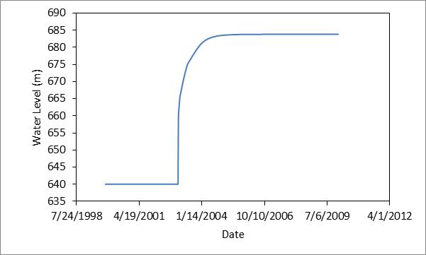
Figure 2.41 Pit-lake level changes through time

Pumping Wells – Discharge vs. Time

Discharge through time from pumping wells is recorded in the “*.FLW” file by MINEDW. The discharge rate for “Pumping with LPE” or “Specified Head” wells, unlike “Pumping Rate” wells, is calculated during the model run. To plot pumping-rate data through time, import the “*.FLW” file into Microsoft^® Excel or other plotting software and select the data for the desired pumping wells.

Particle Tracking

Particle tracking can be used to determine the capture zone of a well or the fate of groundwater within a zone of interest. To evaluate the capture zone of a well, backward particle tracking should be used, while forward particle tracking can be used to predict the fate of groundwater within a zone of interest. The examples provided below and in the “INPUT/PARTICLE TRACKING” directory employ both forward and reverse particle tracking.

To set up reverse particle tracking, choose points along the well screen of any one of the simulated pumping wells. The “INPUT/PARTICLE TRACKING” directory contains two files, “P9_points.DAT” and “P15_points.DAT,” that contain points centered along the simulated screens for two pumps in this tutorial that can be used as a starting point to construct reverse particle tracks. Open the “Particle Tracking” dialog box by clicking on “Results” on the Main Menu banner and selecting “Particle Tracking.” For each of the fields in the “Particle Tracking” dialog box, enter the values shown in Figure 2.42. Alternatively, an input file containing all of the necessary parameters for particle tracking is included in the “INPUT/PARTICLE TRACKING” directory. To use this file to populate the required fields in the “Particle Tracking” dialog box, click on “Open” at the bottom center of the dialog box. Navigate to the location of the “INPUT/PARTICLE TRACKING” directory using the “Open Particle Tracking File” dialog box, select the file “P9 & P15_INPUT (reverse).dat,” and click “Open.” The “Particle Tracking” dialog box should now appear with all the fields filled in except “Result Output,” as shown in Figure 2.42. Enter a file name for the output or, to select a different directory from “INPUT/PARTICLE TRACKING” in which to create the output file, click on the button above and browse to the desired location. Once the output file name and/or directory have been specified, click “OK” at the bottom of the “Particle Tracking” dialog box to begin the particle tracking calculations.

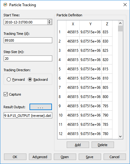
Figure 2.42 Parameters for reverse particle tracking from a pumping well

Once MINEDW has finished the particle tracking calculations, the particle tracks can be visualized in the View Pane by adding a “Particle Tracking” plot item. From the “List” tab in the “Control Panel” pane, double-click on “Post Processing” and then double-click on “Particle Tracking.” Click on the empty field next to the “File” attribute on the “Attributes” tab for the “Particle Tracking” plot item. Using the “Select particle tracking file” dialog box that opens, navigate to the location where the particle tracking file was created by MINEDW, select the file, and click “Open.”

The particle tracks may not immediately display depending on the currently selected time step. Using the time-step slider at the top of MINEDW, change the time step to the date selected as the start date for the reverse particle tracks. Results similar to those shown in Figure 2.43 below should display. This same process can be followed to evaluate the capture zone of any one of the wells used in a simulation.

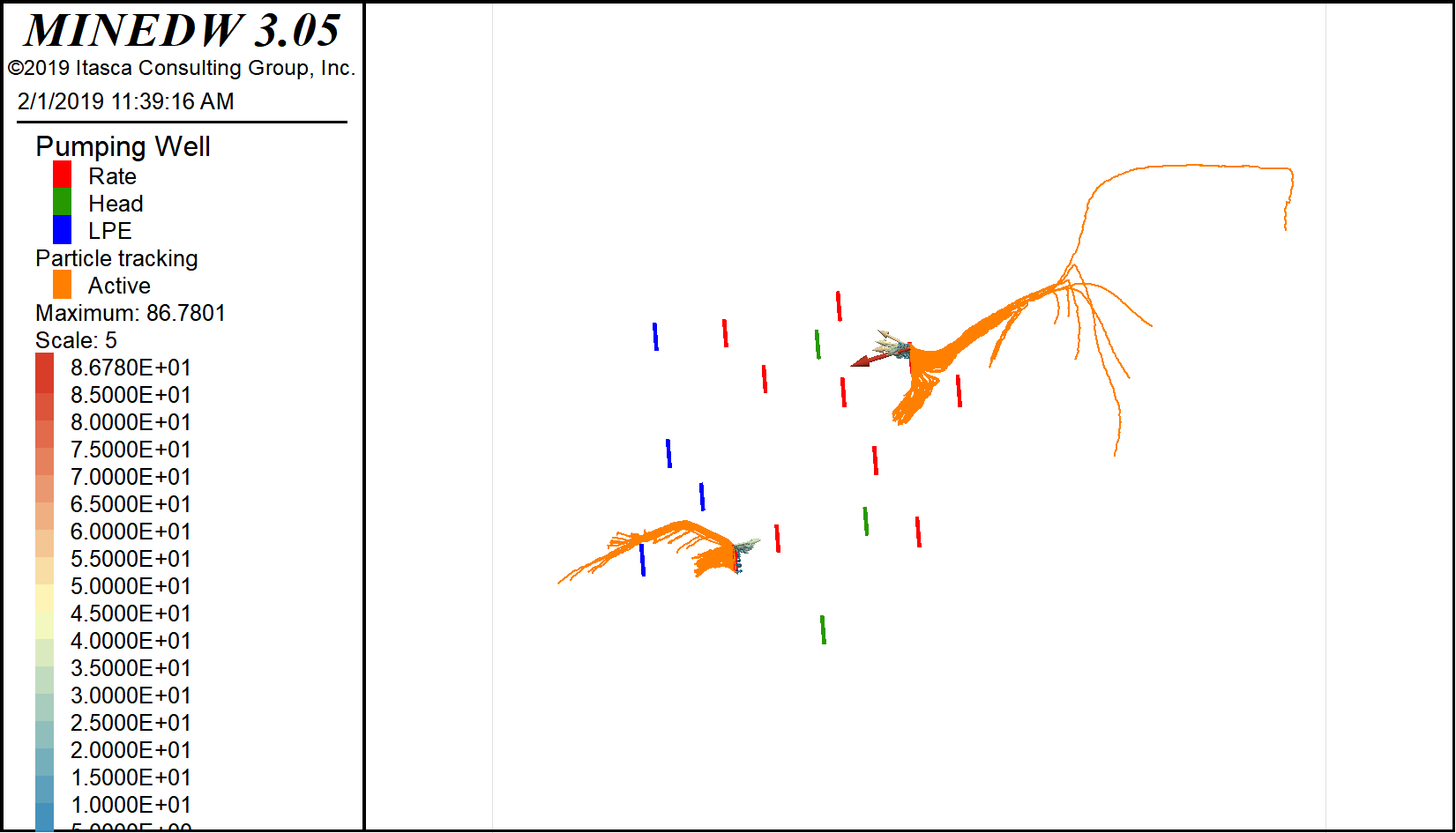
Figure 2.43 Reverse particle tracking results for two pumping wells

Forward particle tracking can be used to evaluate if groundwater from a particular region is captured by pumping wells in the model. To perform forward particle tracking, locate the file named “Region_points.dat” in the directory INPUT/PARTICLE TRACKING. This file contains a group of points located slightly upgradient of the pumping well field in this tutorial. For simplicity, use these points and the particle tracking input file named “Region_INPUT (forward).dat” to populate the “Particle Tracking” dialog box as described in the previous example. Once all of the fields of the “Particle Tracking” dialog box have been filled in, run the particle tracking calculation by clicking “OK.” Next, add a “Particle Tracking” plot item to the View Pane and select the recently created particle track file. Figure 2.44 shows the results of particle tracking for the points in the “Region_INPUT (forward).dat” file.

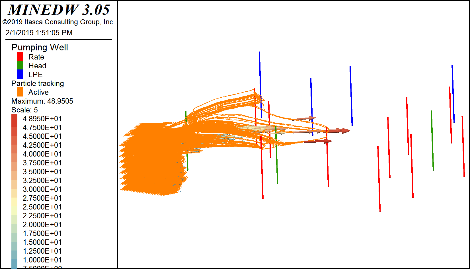
Figure 2.44 Forward particle tracks for an area upgradient of the simulated well field

Only the particles placed within the zones of higher hydraulic conductivity are captured by the pumping wells. The lower geologic units have hydraulic conductivities several orders of magnitude lower than the upper units. Repeat the particle tracking exercise for any desired location by repeating the steps described above.